Problem set 2

due Monday, September 15, 2025 at 11:59am (noon!)

Instructions: Upload your .ipynb notebook to gradescope by 11:59am on the due date. Please include your name, Problem set number, and any collaborators you worked with in a text cell at the top of your notebook. Please also number your problems in some way and include comments in your code to indicate what part of a problem you are working on.
Get help!: If you need support working on your pset, see our week at a glance schedule for office hours and pset support times!

Warning: Avoid redundant loading

You will need the tidyverse library. Recall that Colab comes with this library already installed, and tidyverse includes tibble, readr, and ggplot. Avoid redundant loading.

Problem 1

Create the following tibble with the tribble() function (not tibble()). Use the map() function from the purr package to calculate the median of each column, and store it as col_means. Use the pipe operator (%>% or |>) to pipe that list into as_tibble(), so the output is formatted as tibble. Finally, use rename() to rename the columns of your new tibble to mean_height, mean_weight, and mean_age. Return or print the resulting tibble.

# A tibble: 8 × 3
  height weight   age
   <dbl>  <dbl> <dbl>
1    150     45    18
2    160     54    21
3    165     60    25
4    170     68    30
5    175     72    34
6    180     79    40
7    185     85    50
8    190     90    60

Problem 2

Download this google sheet as a CSV file and upload it into Colab. Then, use the appropriate function from the readr package to import your CSV file into R. Use the na argument to the function to make sure R can recognize the NA values in the RT_ms column. Also include the col_types() argument to the function to ensure the is_frequent column is logical and RT_ms is a double. Use problems() to return the problematic rows in the data. Repair the problems, then use the rename() function to ensure consistent naming in your columns (use _ not spaces).

Problem 3

Sometimes the best way to learn a new package or function is to explore the documentation. The googlesheets4 package allows you to work with Google Sheets directly from R. Read the documentation for this package and figure out how to connect to a sheet, read its contents, and bring the data into R. Use googlesheets4 to import the Europe tab of the gapminder sheet, available here. Return or print the imported sheet to confirm it was read in correctly. You should see the following output.

✔ Reading from "gapminder".

✔ Range ''Europe''.

# A tibble: 360 × 6
   country continent  year lifeExp     pop gdpPercap
   <chr>   <chr>     <dbl>   <dbl>   <dbl>     <dbl>
 1 Albania Europe     1952    55.2 1282697     1601.
 2 Albania Europe     1957    59.3 1476505     1942.
 3 Albania Europe     1962    64.8 1728137     2313.
 4 Albania Europe     1967    66.2 1984060     2760.
 5 Albania Europe     1972    67.7 2263554     3313.
 6 Albania Europe     1977    68.9 2509048     3533.
 7 Albania Europe     1982    70.4 2780097     3631.
 8 Albania Europe     1987    72   3075321     3739.
 9 Albania Europe     1992    71.6 3326498     2497.
10 Albania Europe     1997    73.0 3428038     3193.
# ℹ 350 more rows

Problem 4

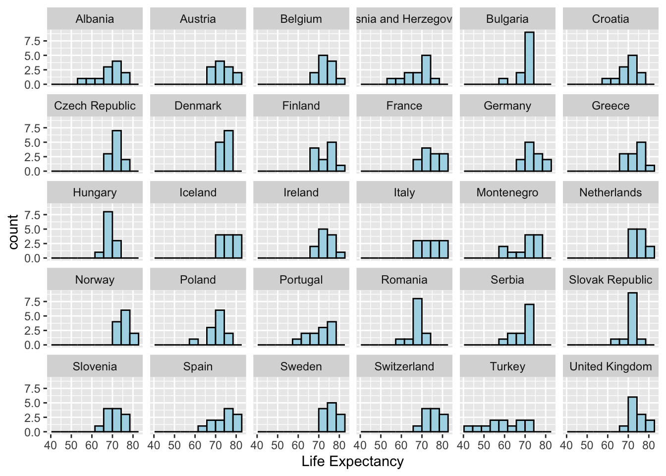
With ggplot2 and the europe data you imported in problem 3, recreate (as faithfully as possible), the following histogram of life expectancy for countries in Europe. Make sure the bars of the histogram are light blue, the border around the bars are black, and you edit the x-axis label to match. Also make sure you have approximately the same number of bins in your histogram.

Using the english dataset in the languageR library, recreate the following table. Convert the dataest to a tibble with as_tibble(), then chain together dplyr verbs with the %>% operator to create the columns in the order shown. Explore the %in%operator and use it with filter in order to filter to the specific words shown. Sort them in alphabetical order, as shown. Use mutate to create two new columns not in the original data: RTnaming_mean (mean of the RTnaming vector) and RTnaming_diffmean (subtract RTnaming_mean from RTnaming)

Word	WordCategory	AgeSubject	LengthInLetters	RTnaming	RTnaming_mean	RTnaming_meandiff
breeze	N	young	6	6.119858	6.320535	-0.2006769
breeze	N	old	6	6.472964	6.320535	0.1524297
moose	N	young	5	6.123370	6.320535	-0.1971650
moose	N	old	5	6.542760	6.320535	0.2222255
owl	N	young	3	6.153158	6.320535	-0.1673765
owl	N	old	3	6.459905	6.320535	0.1393698
pup	N	young	3	6.135998	6.320535	-0.1845369
pup	N	old	3	6.485551	6.320535	0.1650162
queen	N	young	5	6.181051	6.320535	-0.1394833
queen	N	old	5	6.530732	6.320535	0.2101972

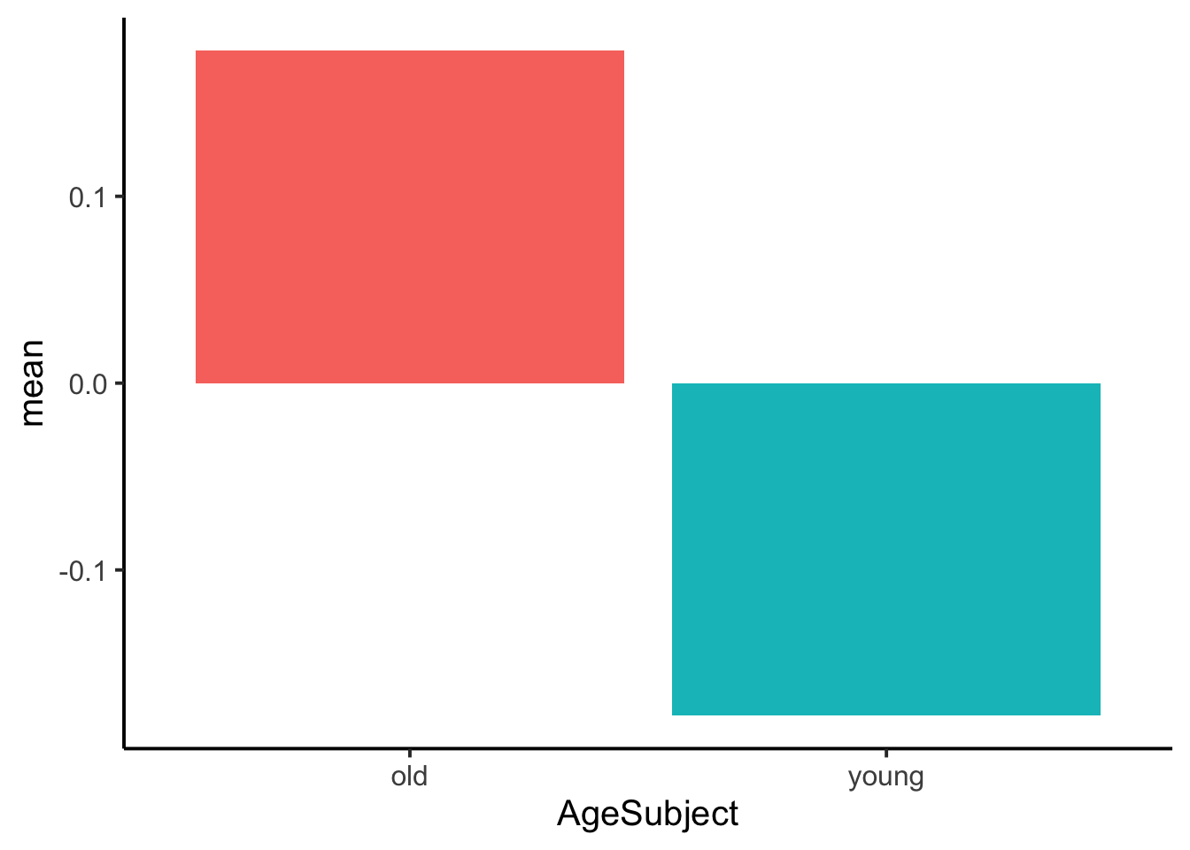
Take the resulting tibble from question 5, group the data by AgeSubject with group_by() and summarise() by computing the mean and standard deviation ofRTnaming_mean. Return the summarized tibble or print it (as shown). Then use the summarized data to recreate the figure. Figure out how to remove the legend entirely!

AgeSubject	mean	sd
old	0.1778477	0.0364251
young	-0.1778477	0.0251025