Model Specification

Data Science for Studying Language and the Mind

Katie Schuler

Tuesday

Announcements

You are `here`

Data science with R

R basics
Data visualization
Data wrangling

Stats & Model building

Sampling distribution
Hypothesis testing
Model specification
Model fitting
Model accuracy
Model reliability

More advanced

Classification

Review

Sampling distribution and hypothesis testing with Correlation!

Exploring relationships

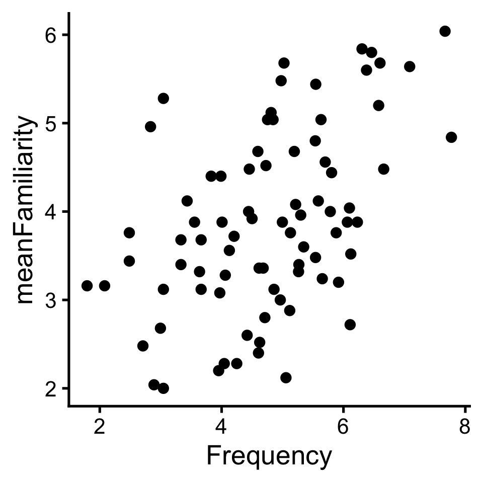
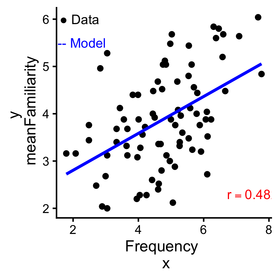
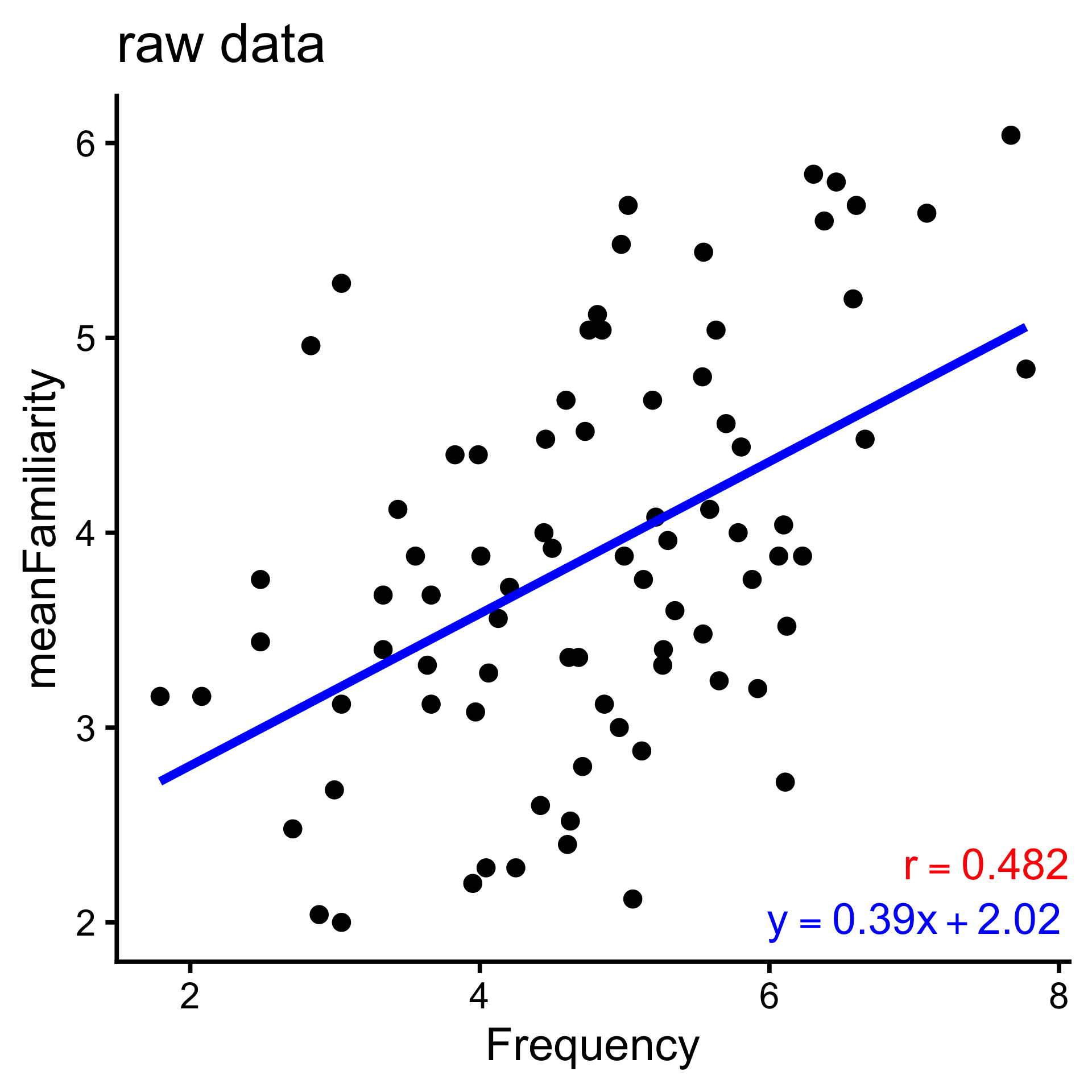
To review what we learned before break, let’s explore the relationship between Frequency and meanFamiliarity in the ratings dataset of the languageR package.

Is there a relationship?

If there was no relationship, we’d say there are independent: knowing the value of one provides no information about about the other. But that’s not the case here.

Yes, a linear relationship

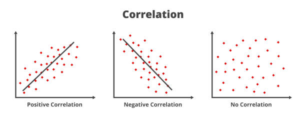
In a linear relationship, when one variable goes up the other goes up (positive); or when one goes up the other goes down (negative).

Quantify with correlation

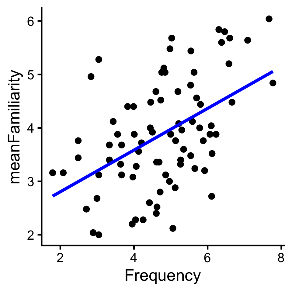
One way to quantify linear relationships is with correlation ($r$). Correlation expresses the linear relationship as a range from -1 (perfectly negative) to 1 (perfectly positive).

Computing correlation in R

We can compute a correlation with R’s built in cor(x,y) function

cor(
  x = ratings$Frequency, 
  y = ratings$meanFamiliarity
)

[1] 0.4820286

Or via the infer pacakge.

(obs_corr <- ratings %>%
  specify(
    response = meanFamiliarity, 
    explanatory = Frequency
  ) %>%
  calculate(stat = "correlation"))

Response: meanFamiliarity (numeric)
Explanatory: Frequency (numeric)
# A tibble: 1 × 1
   stat
  <dbl>
1 0.482

Correlation uncertainty

Just like the mean — and all other test statistics! — $r$ is subject to sampling variability. We can indicate our uncertainty around the correlation the same way we always have:

Construct the sampling distribution for the correlation:

sampling_distribution <- ratings %>%
  specify(
    response = meanFamiliarity, 
    explanatory = Frequency
  ) %>%
  generate(reps = 1000, type = "bootstrap") %>%
  calculate(stat = "correlation")

head(sampling_distribution)

Response: meanFamiliarity (numeric)
Explanatory: Frequency (numeric)
# A tibble: 6 × 2
  replicate  stat
      <int> <dbl>
1         1 0.444
2         2 0.595
3         3 0.533
4         4 0.565
5         5 0.573
6         6 0.579

Compute a confidence interval

ci <- sampling_distribution %>% 
  get_ci(level = 0.95, type = "percentile")

ci

# A tibble: 1 × 2
  lower_ci upper_ci
     <dbl>    <dbl>
1    0.305    0.635

💪 In-class Exercise

Take a few minutes to try this yourself!

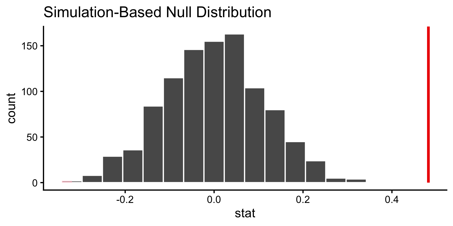
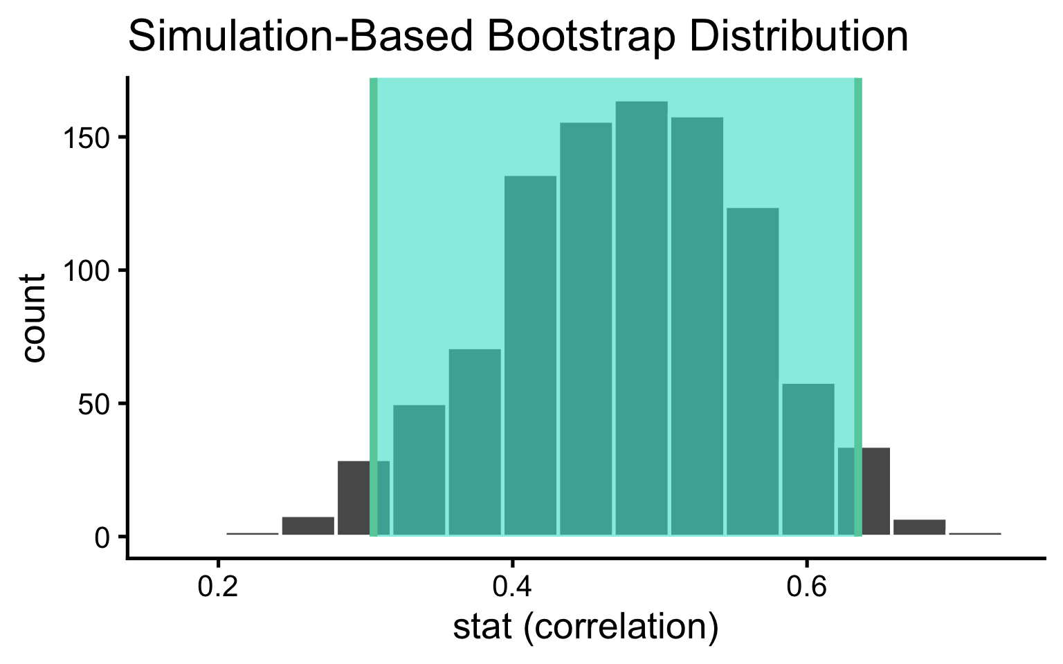
Use the infer way to visualize the sampling distribution and shade the confidence interval we just computed. Change the x-axis label to stat (correlation) as pictured below.

Hypothesis testing our correlation

How do we test whether the correlation we observed is significantly different from zero? Hypothesis test!

Step 1: Construct the null distribution, the sampling distribution of the null hypothesis

null_distribution_corr <- ratings %>% 
  specify(
    response = meanFamiliarity, 
    explanatory = Frequency
  ) %>%
  hypothesize(null = "independence") %>%
  generate(reps = 1000, type = "permute") %>%
  calculate(stat = "correlation") 

null_distribution_corr %>% head

Response: meanFamiliarity (numeric)
Explanatory: Frequency (numeric)
Null Hyp...
# A tibble: 6 × 2
  replicate    stat
      <int>   <dbl>
1         1 -0.189 
2         2  0.0233
3         3 -0.0523
4         4 -0.0187
5         5 -0.0674
6         6 -0.0242

Step 2: How likley is our observed value under the null? Get a p-value.

p <- null_distribution_corr %>%
  get_p_value(
    obs_stat = obs_corr, 
    direction = "both")
p

# A tibble: 1 × 1
  p_value
    <dbl>
1       0

Hypothesis testing our correlation

How do we test whether the correlation we observed is significantly different from zero? Hypothesis test!

Step 3: Decide whether to reject the null!

null_distribution_corr %>% 
  visualize() + 
  shade_p_value(
    obs_stat = obs_corr, 
    direction = "two-sided"
  )

Interpret our p-value. Should we reject the null hypothesis?

Model building

Big picture overview of the model building process and the types of models we might encounter in our research.

Correlation is model building

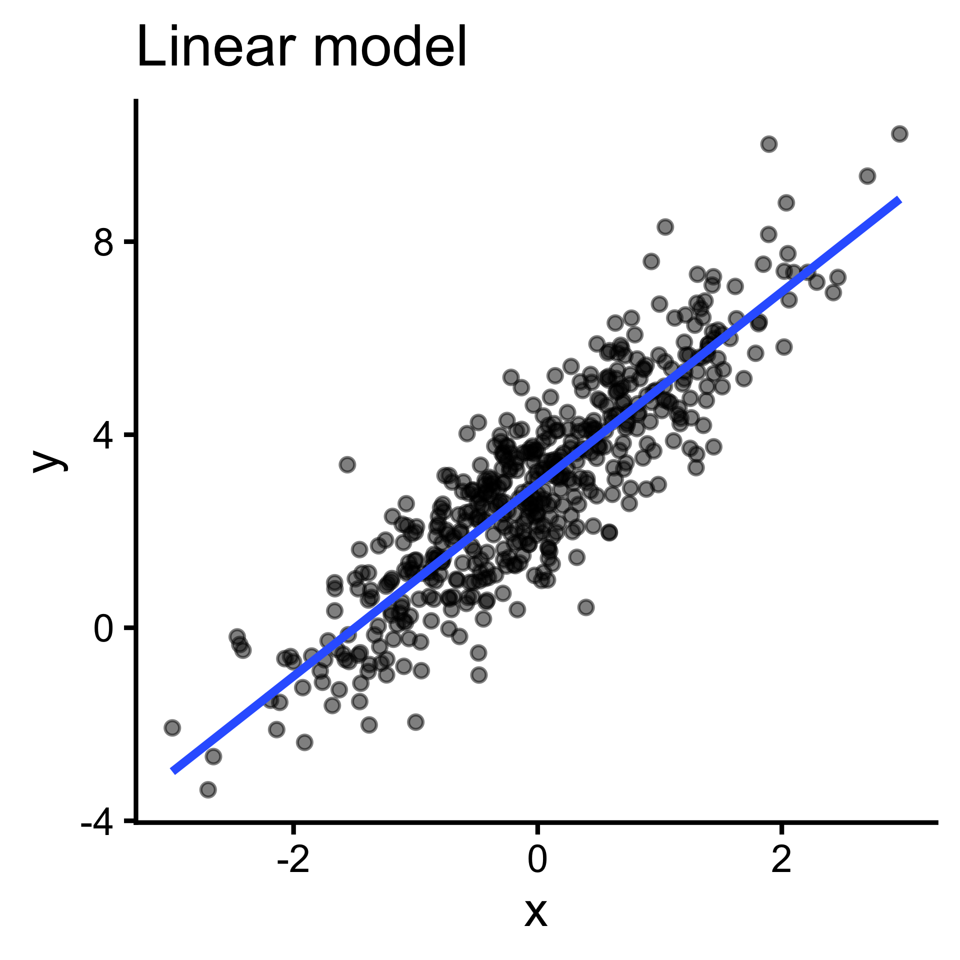
Correlation is a simple case of model building, in which we use one value ($x$) to predict another ($y$).

Correlation is model building

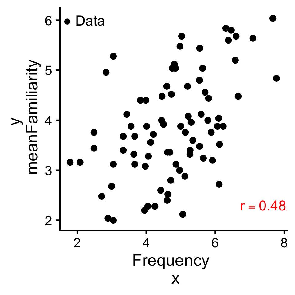
Even more specifically — formally, the model specification — we are fitting the linear model $y = ax+b$, where $a$ and $b$ are free parameters.

Model specification: $y = ax + b$
Estimate free parameters: $a$ and $b$
Fitted model: $y = 0.39x + 2.02$

How do we get $r = 0.48$ ?

The link between correlation and linear models is understood when we normalize our variables with a z-score.

z_ratings <- ratings %>%
  select(Frequency, meanFamiliarity) %>%
  mutate(
    z_Freq = scale(Frequency), 
    z_meanFamil = scale(meanFamiliarity)
  )

z_ratings %>% head

  Frequency meanFamiliarity     z_Freq z_meanFamil
1  4.204693            3.72 -0.4387602  -0.1573220
2  5.347108            3.60  0.4619516  -0.2742310
3  6.304449            5.84  1.2167459   1.9080703
4  3.828641            4.40 -0.7352500   0.5051623
5  3.663562            3.68 -0.8654029  -0.1962917
6  3.433987            4.12 -1.0464062   0.2323747

A z-score gets the number of standard deviations a data point is from the mean.

Correlation is the slope of the model

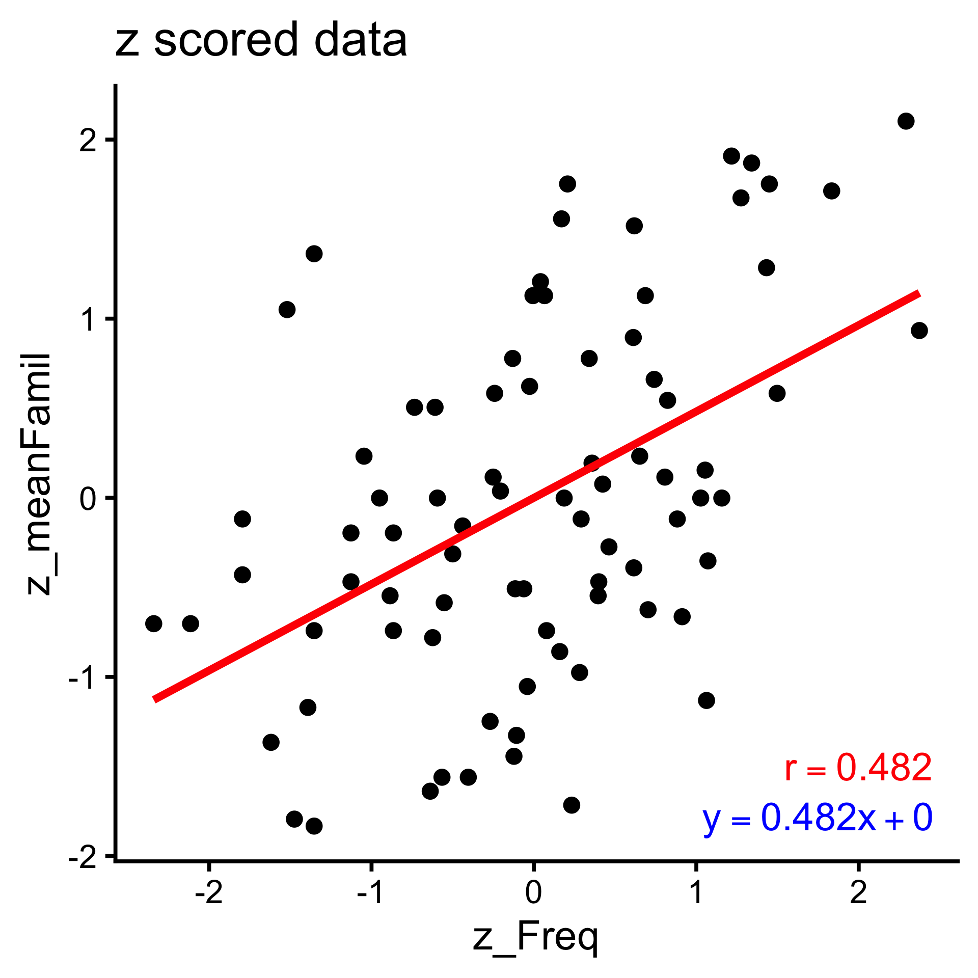
Correlation is the slope of the line that best predicts $y$ from $x$ (after z-scoring)

Model building overview

Model specification (this week): specify the functional form of the model.
Model fitting: you have the form, how do you estimate the free parameters?
Model accuracy: you’ve estimated the parameters, how well does that model describe your data?
Model reliability: when you estimate the parameters, you want to quantify your uncertainty on your estimates

Types of models

💪 In-class Exercise

Take a few minutes to try this yourself!

Ask ChatGPT what type of model it is made with?

Supervised learning

Types of models

Regression v classification

Types of models

Linear models

Linear models are models in which the output (y) is a weighted sum of the inputs
Easy to understand and fit
$y=\sum_{i=1}^{n}w_ix_i$
$y = ax + b$ is this!

Linear model equation

$y = ax + b$ can be expressed $y=\sum_{i=1}^{n}w_ix_i$

Types of models

Nonlinear models

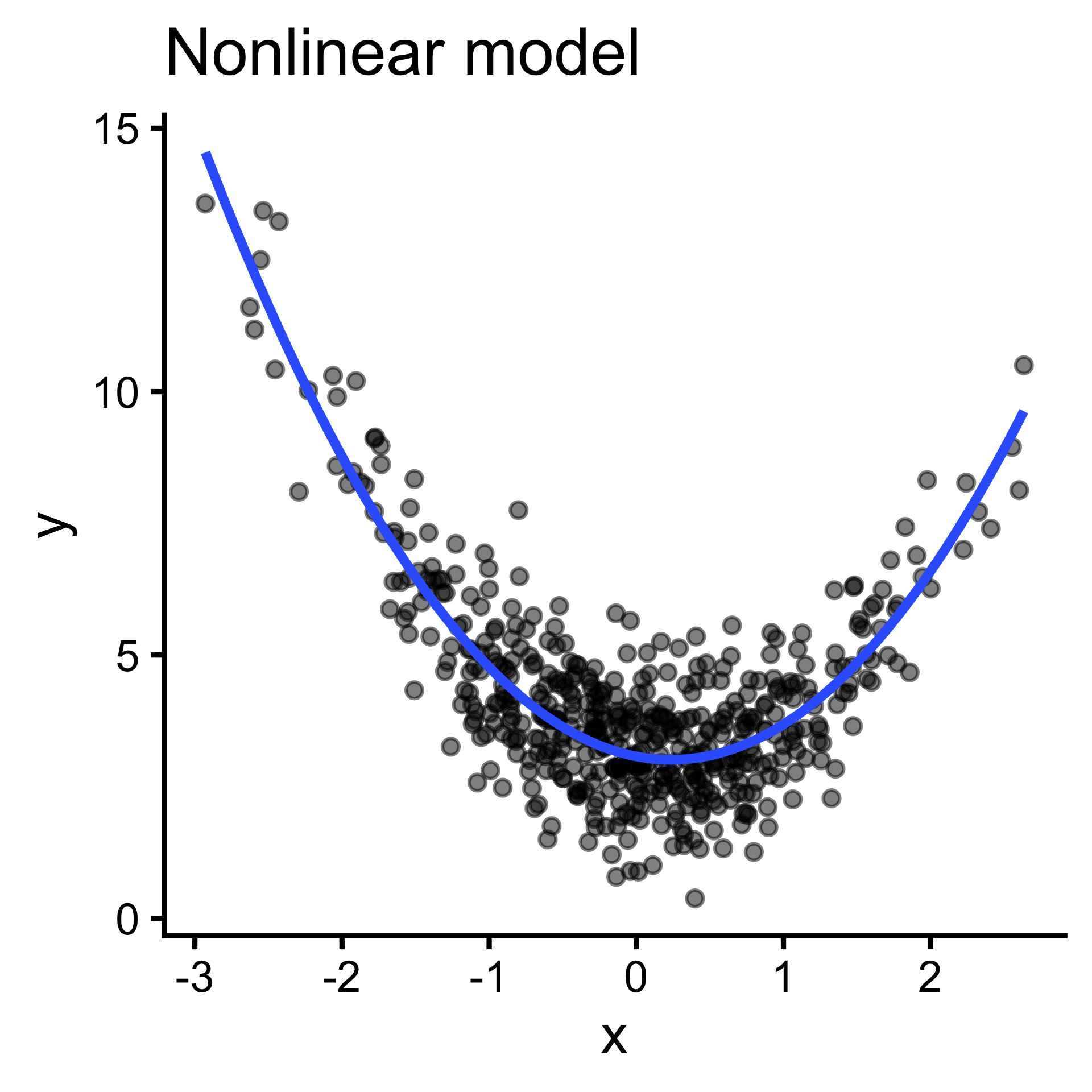
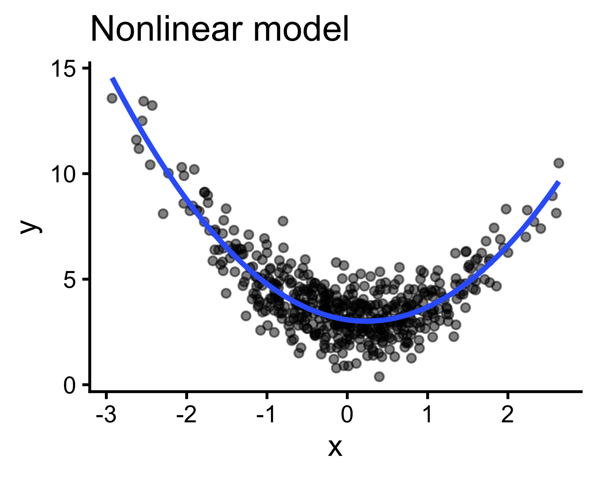
Output (y) cannot be expressed as a weighted sum of inputs($y=\sum_{i=1}^{n}w_ix_i$ ); pattern is better captured by more complex functions. (But often we can linearize them!)

💪 In-class Exercise

Take a few minutes to try this yourself!

Load the following data, which shows brain size and body weight for several different animals:

animal_brain_body_size.csv

Explore the data to specify the type of model we should use to predict brain size by body weight.

Supervised or unsupervised?
Regression or classification?
Linear or nonlinear?

Model specification

Recall that model specification is one aspect of the model building process in which we select the form of the model (the type of model)

Response variable ($y$): Specify the variable you want to predict/explain (output).
Explanatory variables($x_i$): Specify the variables that may explain the variation in the response (inputs).
Functional form: Specify the relationship between the response and explanatory variables. For linear models, we use the linear model equation!
Model terms: Specify how to include your explanatory variables in the model (since they can be included in more than one way).

Model specification

The following issues can also be considered part of the model specification process.

Model assumptions: Check any assumptions underlying the model you selected (e.g. does the model assume the relationship is linear?).
Model complexity: Simple models are easier to interpret but may not capture all complexities in the data. Complex models may suffer from overfitting the data or being difficult to interpret.

A well-specified model should be based on a clear understanding of the data, the underlying relationships, and the research question.

Specifying the functional form

Literally specifying the mathematical formula we’re going to use to represent the relationship between our response and explanatory variables.
We already know it: linear models are models in whch the response variable ($y$) is a weighted sum of the explanatory variables ($x_i$)
$y=\sum_{i=1}^{n}w_ix_i$

🥸 Aliases of $y=\sum_{i=1}^{n}w_ix_i$

The linear model equation can be expressed in many ways, but they are all this same thing

in high school algebra: $y=ax+b$.
in machine learning: $y = w_0 + w_1x_1 + w_2x_2 + ... + w_nx_n$
in statistics: $y = β_0 + β_1x_1 + β_2x_2 + ... + β_nx_n + ε$
in matrix notation: $y = Xβ + ε$

Specify our first model

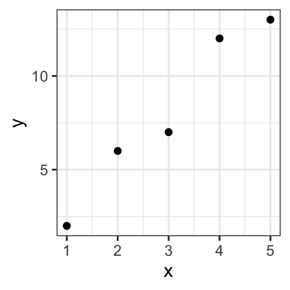
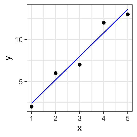
To illustrate how this simple equation scales up to complex models, let’s start with a simple case (“toy”, “tractable”).

# A tibble: 2 × 2
      x     y
  <dbl> <dbl>
1     1     3
2     2     5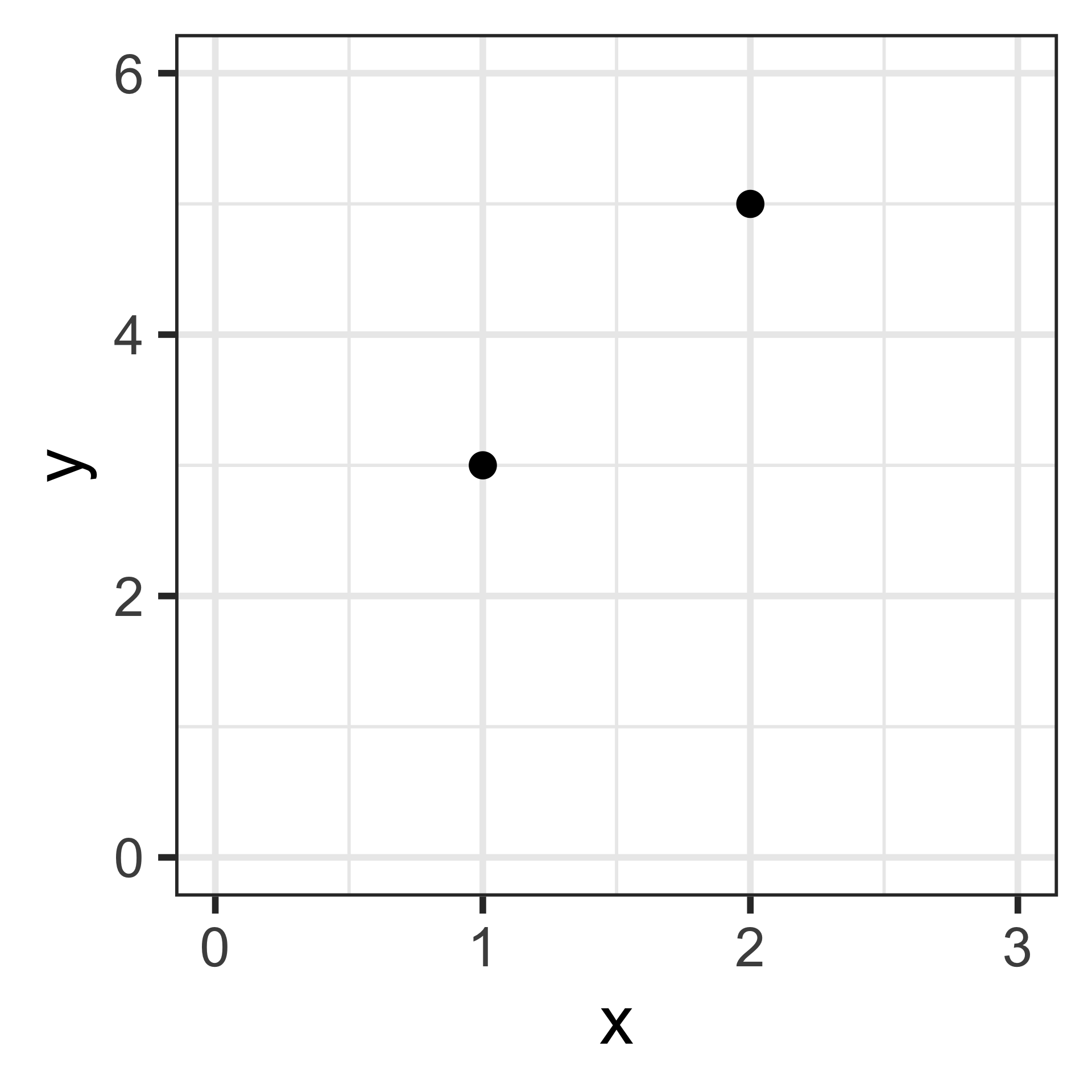

💪 In class exercise

Specify our model!

Swim Records

Applied to a more complex problem

Specify a model for `SwimRecords`

How have world swim records in the 100m changed over time?

library(mosaic)
glimpse(SwimRecords)

Rows: 62
Columns: 3
$ year <int> 1905, 1908, 1910, 1912, 1918, 1920, 1922, 1924, 1934, 1935, 1936,…
$ time <dbl> 65.80, 65.60, 62.80, 61.60, 61.40, 60.40, 58.60, 57.40, 56.80, 56…
$ sex  <fct> M, M, M, M, M, M, M, M, M, M, M, M, M, M, M, M, M, M, M, M, M, M,…

💪 In class exercise

Plot the swim records data, then use your model specification worksheet to specify the model.

Response variable $y$

What is the thing you are trying to understand?

Explanatory variable(s) $x_i$

What could explain the variation in your response variable?

year
year + sex

Functional form

Linear model
$y=\sum_{i=1}^{n}w_ix_i$

Model terms

Model terms describe how to include our explanatory variables in our model formula — there is more than one way!

Intercept
Main
Interaction
Transformation

Intercept

in R: y ~ 1, in eq: $y=w_1x_1$

in R: y ~ 1 + year, in eq: $y = w_1x_1 + w_2x_2$

in R: y ~ 1 + sex, in eq: $y = w_1x_1 + w_2x_2$

in R: y ~ 1 + year, in eq: $y = w_1x_1 + w_2x_2 + w_3x_3$

Interaction

in R: y ~ 1 + year + gender + year:gender
- or the short way: y ~ 1 + year * gender
in eq: $y = w_1x_1 + w_2x_2 + w_3x_3 + w_4x_4$ where $x_4$ is $x_2x_3$

Transformation

in R: y ~ 1 + year * sex + I(year^2)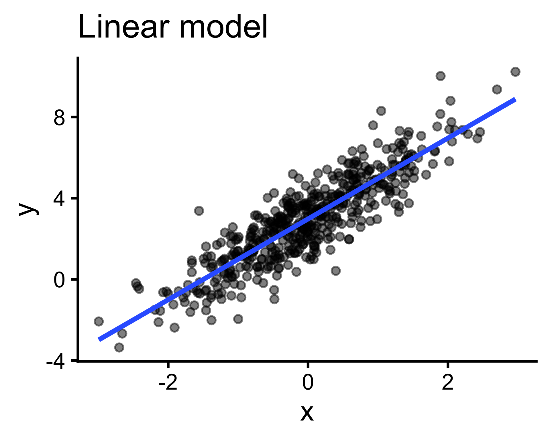
in eq: $y = w_1x_1 + w_2x_2 + w_3x_3 + w_4x_4$ + $w_5x_5$
- where $x_4$ is $x_2x_3$ and $x_5$ is $x_2^2$

THursday

Model building overview

Model specification (this week): specify the functional form of the model.
Model fitting: you have the form, how do you estimate the free parameters?
Model accuracy: you’ve estimated the parameters, how well does that model describe your data?
Model reliability: when you estimate the parameters, you want to quantify your uncertainty on your estimates

Types of models

Regression v classification

Linear v Nonlinear models

Linear models output ($y$) is a weighted sum of inputs ($x_i$): $y=\sum_{i=1}^{n}w_ix_i$
Nonlinear models cannot be expressed as a weighted sum of inputs
- but usually we can linearize them!

Model specification

First aspect of the model building process in which we select the form of the model (the type of model)

Response variable ($y$): Specify the variable you want to predict/explain (output).
Explanatory variables($x_i$): Specify the variables that may explain the variation in the response (inputs).
Functional form: Specify the relationship between the response and explanatory variables: $y=\sum_{i=1}^{n}w_ix_i$
Model terms: Specify how to include your explanatory variables in the model (since they can be included in more than one way).

“Toy” data

toy_data <- tibble(
  x = c(1, 2, 3, 4, 5), 
  y = c(2, 6, 7, 12, 13)
)

Explore the data

Plot
Data
Code

x	y
1	2
2	6
3	7
4	12
5	13

toy_data <- tibble(
  x = c(1, 2, 3, 4, 5), 
  y = c(2, 6, 7, 12, 13)
)

toy_data %>%
  ggplot(aes(x = x, y = y)) +
  geom_point() +
  theme_bw(base_size = 14)

💪In-class exercise

Specify a model for the toy data. Then use lm() to fit the model.

Specify, fit, plot model

Plot
Data
Code

Model specification:
$y = w_1\cdot\mathbf{1} + w_2\cdot\mathbf{x}$


Call:
lm(formula = y ~ 1 + x, data = toy_data)

Coefficients:
(Intercept)            x  
       -0.4          2.8

Fitted model:
$y = -0.4\cdot1 + 2.8\cdot x$

x	y	with_formula	with_predict
1	2	2.4	2.4
2	6	5.2	5.2
3	7	8.0	8.0
4	12	10.8	10.8
5	13	13.6	13.6

model <- lm(y ~ 1 + x, data = toy_data)

toy_data <- toy_data %>%
  mutate(with_formula = -0.4*1 + 2.8*x) %>%
  mutate(with_predict= predict(model, toy_data))

toy_data %>%
  ggplot(aes(x = x, y = y)) +
  geom_point() +
  geom_line(aes(y = with_predict), color = "blue") +
  theme_bw(base_size = 14)

Swim records

library(mosaic)

One input

Plot
Data
Code

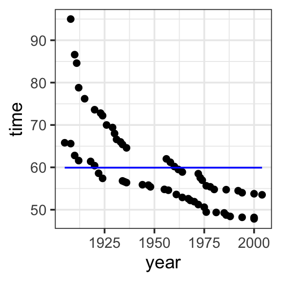
Model specification:
$y = w_1\cdot\mathbf{1}$


Call:
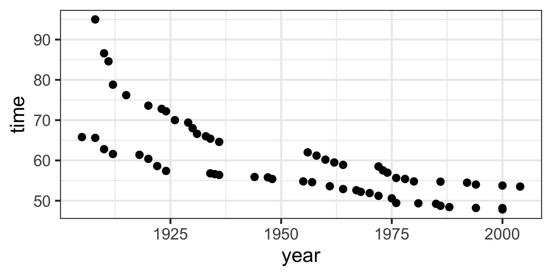
lm(formula = time ~ 1, data = SwimRecords)

Coefficients:
(Intercept)  
      59.92

Fitted model:
$y = 59.92 \cdot 1$

year	time	sex	with_formula	with_predict
1905	65.80	M	59.92	59.92419
1908	65.60	M	59.92	59.92419
1910	62.80	M	59.92	59.92419
1912	61.60	M	59.92	59.92419
1918	61.40	M	59.92	59.92419
1920	60.40	M	59.92	59.92419
1922	58.60	M	59.92	59.92419
1924	57.40	M	59.92	59.92419
1934	56.80	M	59.92	59.92419
1935	56.60	M	59.92	59.92419
1936	56.40	M	59.92	59.92419
1944	55.90	M	59.92	59.92419
1947	55.80	M	59.92	59.92419
1948	55.40	M	59.92	59.92419
1955	54.80	M	59.92	59.92419
1957	54.60	M	59.92	59.92419
1961	53.60	M	59.92	59.92419
1964	52.90	M	59.92	59.92419
1967	52.60	M	59.92	59.92419
1968	52.20	M	59.92	59.92419
1970	51.90	M	59.92	59.92419
1972	51.22	M	59.92	59.92419
1975	50.59	M	59.92	59.92419
1976	49.44	M	59.92	59.92419
1981	49.36	M	59.92	59.92419
1985	49.24	M	59.92	59.92419
1986	48.74	M	59.92	59.92419
1988	48.42	M	59.92	59.92419
1994	48.21	M	59.92	59.92419
2000	48.18	M	59.92	59.92419
2000	47.84	M	59.92	59.92419
1908	95.00	F	59.92	59.92419
1910	86.60	F	59.92	59.92419
1911	84.60	F	59.92	59.92419
1912	78.80	F	59.92	59.92419
1915	76.20	F	59.92	59.92419
1920	73.60	F	59.92	59.92419
1923	72.80	F	59.92	59.92419
1924	72.20	F	59.92	59.92419
1926	70.00	F	59.92	59.92419
1929	69.40	F	59.92	59.92419
1930	68.00	F	59.92	59.92419
1931	66.60	F	59.92	59.92419
1933	66.00	F	59.92	59.92419
1934	65.40	F	59.92	59.92419
1936	64.60	F	59.92	59.92419
1956	62.00	F	59.92	59.92419
1958	61.20	F	59.92	59.92419
1960	60.20	F	59.92	59.92419
1962	59.50	F	59.92	59.92419
1964	58.90	F	59.92	59.92419
1972	58.50	F	59.92	59.92419
1973	57.54	F	59.92	59.92419
1974	56.96	F	59.92	59.92419
1976	55.65	F	59.92	59.92419
1978	55.41	F	59.92	59.92419
1980	54.79	F	59.92	59.92419
1986	54.73	F	59.92	59.92419
1992	54.48	F	59.92	59.92419
1994	54.01	F	59.92	59.92419
2000	53.77	F	59.92	59.92419
2004	53.52	F	59.92	59.92419

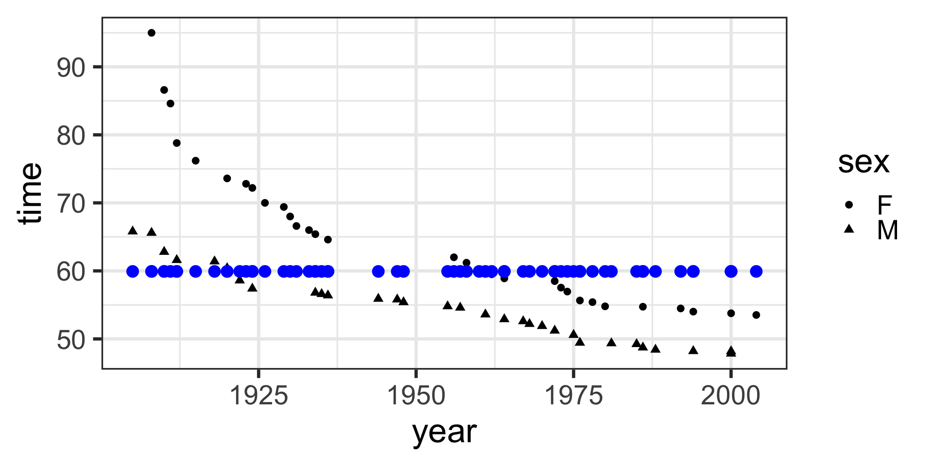
model <- lm(time ~ 1, data = SwimRecords)

SwimRecords_predict <- SwimRecords %>%
  mutate(with_formula = 59.92*1) %>% 
  mutate(with_predict= predict(model, SwimRecords))

SwimRecords_predict %>%
  ggplot(aes(x = year, y = time)) +
  geom_point() +
  geom_line(aes(y = with_predict), color = "blue") +
  theme_bw(base_size = 14)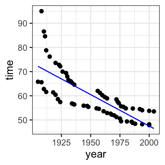

💪In-class exercise

Specify a model for the SwimRecords data that includes the intercept and the year. Use lm() to fit the model. Then use predict() to get the models prediction.

If you have time, plot the data and model predictions with ggplot().

Two inputs

Plot
Data
Code

Model specification:
$y = w_1\cdot\mathbf{1} + w_2\cdot\mathbf{year}$


Call:
lm(formula = time ~ 1 + year, data = SwimRecords)

Coefficients:
(Intercept)         year  
   567.2420      -0.2599

Fitted model:
$y = 567.2420 \cdot \mathbf{1} + -0.2599 \cdot \mathbf{year}$

year	time	sex	with_formula	with_predict
1905	65.80	M	72.1325	72.17614
1908	65.60	M	71.3528	71.39651
1910	62.80	M	70.8330	70.87676
1912	61.60	M	70.3132	70.35700
1918	61.40	M	68.7538	68.79774
1920	60.40	M	68.2340	68.27798
1922	58.60	M	67.7142	67.75823
1924	57.40	M	67.1944	67.23848
1934	56.80	M	64.5954	64.63971
1935	56.60	M	64.3355	64.37983
1936	56.40	M	64.0756	64.11995
1944	55.90	M	61.9964	62.04093
1947	55.80	M	61.2167	61.26130
1948	55.40	M	60.9568	61.00143
1955	54.80	M	59.1375	59.18229
1957	54.60	M	58.6177	58.66253
1961	53.60	M	57.5781	57.62302
1964	52.90	M	56.7984	56.84339
1967	52.60	M	56.0187	56.06376
1968	52.20	M	55.7588	55.80388
1970	51.90	M	55.2390	55.28413
1972	51.22	M	54.7192	54.76438
1975	50.59	M	53.9395	53.98474
1976	49.44	M	53.6796	53.72487
1981	49.36	M	52.3801	52.42548
1985	49.24	M	51.3405	51.38597
1986	48.74	M	51.0806	51.12610
1988	48.42	M	50.5608	50.60634
1994	48.21	M	49.0014	49.04708
2000	48.18	M	47.4420	47.48782
2000	47.84	M	47.4420	47.48782
1908	95.00	F	71.3528	71.39651
1910	86.60	F	70.8330	70.87676
1911	84.60	F	70.5731	70.61688
1912	78.80	F	70.3132	70.35700
1915	76.20	F	69.5335	69.57737
1920	73.60	F	68.2340	68.27798
1923	72.80	F	67.4543	67.49835
1924	72.20	F	67.1944	67.23848
1926	70.00	F	66.6746	66.71872
1929	69.40	F	65.8949	65.93909
1930	68.00	F	65.6350	65.67921
1931	66.60	F	65.3751	65.41934
1933	66.00	F	64.8553	64.89958
1934	65.40	F	64.5954	64.63971
1936	64.60	F	64.0756	64.11995
1956	62.00	F	58.8776	58.92241
1958	61.20	F	58.3578	58.40266
1960	60.20	F	57.8380	57.88290
1962	59.50	F	57.3182	57.36315
1964	58.90	F	56.7984	56.84339
1972	58.50	F	54.7192	54.76438
1973	57.54	F	54.4593	54.50450
1974	56.96	F	54.1994	54.24462
1976	55.65	F	53.6796	53.72487
1978	55.41	F	53.1598	53.20511
1980	54.79	F	52.6400	52.68536
1986	54.73	F	51.0806	51.12610
1992	54.48	F	49.5212	49.56683
1994	54.01	F	49.0014	49.04708
2000	53.77	F	47.4420	47.48782
2004	53.52	F	46.4024	46.44831

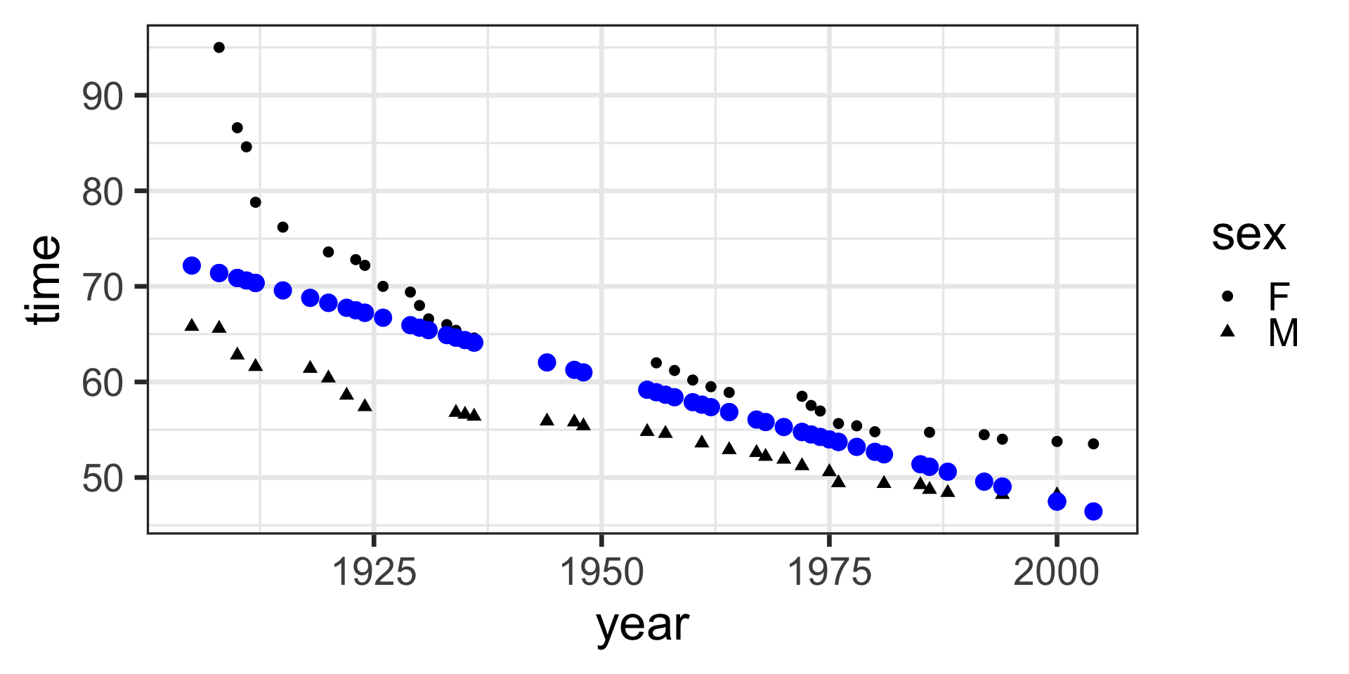
model <- lm(time ~ 1 + year, data = SwimRecords)

SwimRecords_predict <- SwimRecords %>%
  mutate(with_formula = 567.2420*1 + -0.2599*year) %>%
  mutate(with_predict= predict(model, SwimRecords))

SwimRecords_predict %>%
  ggplot(aes(x = year, y = time)) +
  geom_point() +
  geom_line(aes(y = with_predict), color = "blue") +
  theme_bw(base_size = 14)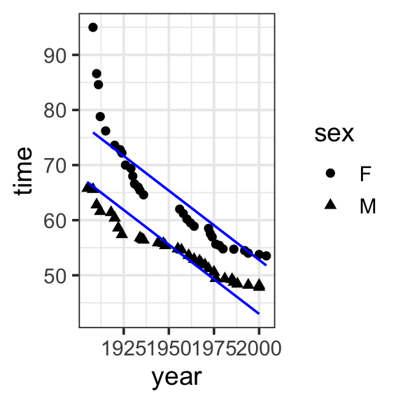

Three inputs

Plot
Data
Code

Model specification:
$y = w_1\cdot\mathbf{1} + w_2\cdot\mathbf{year} + w_3\cdot\mathbf{sex}$


Call:
lm(formula = time ~ 1 + year + sex, data = SwimRecords)

Coefficients:
(Intercept)         year         sexM  
   555.7168      -0.2515      -9.7980

Fitted model:
$y = 555.7168 \cdot \mathbf{1} + -0.2515 \cdot \mathbf{year} + -9.7980 \cdot \mathbf{sex}$

year	time	sex	sex_numeric	with_formula	with_predict
1905	65.80	M	1	66.8113	66.88051
1908	65.60	M	1	66.0568	66.12612
1910	62.80	M	1	65.5538	65.62319
1912	61.60	M	1	65.0508	65.12026
1918	61.40	M	1	63.5418	63.61148
1920	60.40	M	1	63.0388	63.10855
1922	58.60	M	1	62.5358	62.60563
1924	57.40	M	1	62.0328	62.10270
1934	56.80	M	1	59.5178	59.58806
1935	56.60	M	1	59.2663	59.33660
1936	56.40	M	1	59.0148	59.08513
1944	55.90	M	1	57.0028	57.07343
1947	55.80	M	1	56.2483	56.31903
1948	55.40	M	1	55.9968	56.06757
1955	54.80	M	1	54.2363	54.30732
1957	54.60	M	1	53.7333	53.80440
1961	53.60	M	1	52.7273	52.79854
1964	52.90	M	1	51.9728	52.04415
1967	52.60	M	1	51.2183	51.28976
1968	52.20	M	1	50.9668	51.03830
1970	51.90	M	1	50.4638	50.53537
1972	51.22	M	1	49.9608	50.03244
1975	50.59	M	1	49.2063	49.27805
1976	49.44	M	1	48.9548	49.02659
1981	49.36	M	1	47.6973	47.76927
1985	49.24	M	1	46.6913	46.76341
1986	48.74	M	1	46.4398	46.51195
1988	48.42	M	1	45.9368	46.00902
1994	48.21	M	1	44.4278	44.50024
2000	48.18	M	1	42.9188	42.99146
2000	47.84	M	1	42.9188	42.99146
1908	95.00	F	0	75.8548	75.92408
1910	86.60	F	0	75.3518	75.42115
1911	84.60	F	0	75.1003	75.16969
1912	78.80	F	0	74.8488	74.91822
1915	76.20	F	0	74.0943	74.16383
1920	73.60	F	0	72.8368	72.90651
1923	72.80	F	0	72.0823	72.15212
1924	72.20	F	0	71.8308	71.90066
1926	70.00	F	0	71.3278	71.39773
1929	69.40	F	0	70.5733	70.64334
1930	68.00	F	0	70.3218	70.39188
1931	66.60	F	0	70.0703	70.14041
1933	66.00	F	0	69.5673	69.63749
1934	65.40	F	0	69.3158	69.38602
1936	64.60	F	0	68.8128	68.88310
1956	62.00	F	0	63.7828	63.85382
1958	61.20	F	0	63.2798	63.35090
1960	60.20	F	0	62.7768	62.84797
1962	59.50	F	0	62.2738	62.34504
1964	58.90	F	0	61.7708	61.84211
1972	58.50	F	0	59.7588	59.83040
1973	57.54	F	0	59.5073	59.57894
1974	56.96	F	0	59.2558	59.32748
1976	55.65	F	0	58.7528	58.82455
1978	55.41	F	0	58.2498	58.32162
1980	54.79	F	0	57.7468	57.81869
1986	54.73	F	0	56.2378	56.30991
1992	54.48	F	0	54.7288	54.80113
1994	54.01	F	0	54.2258	54.29820
2000	53.77	F	0	52.7168	52.78942
2004	53.52	F	0	51.7108	51.78357

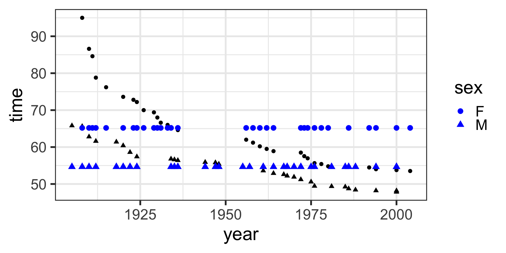
model <- lm(time ~ 1 + year + sex, data = SwimRecords)

SwimRecords_predict <- SwimRecords %>%
  mutate(sex_numeric = case_when(
    sex == 'M' ~ 1,
    sex == 'F' ~ 0
  )) %>%
  mutate(with_formula = 555.7168*1 + -0.2515*year + -9.7980 *sex_numeric) %>%
  mutate(with_predict= predict(model, SwimRecords))

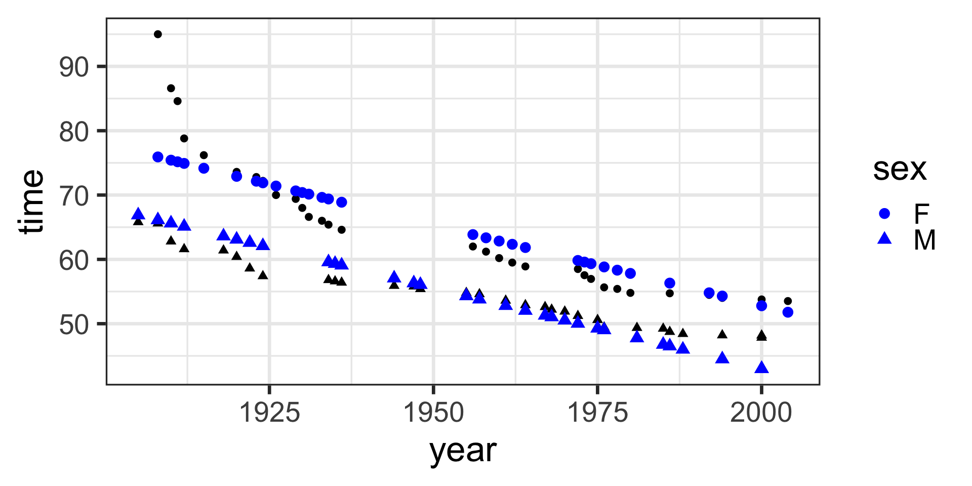
SwimRecords_predict %>%
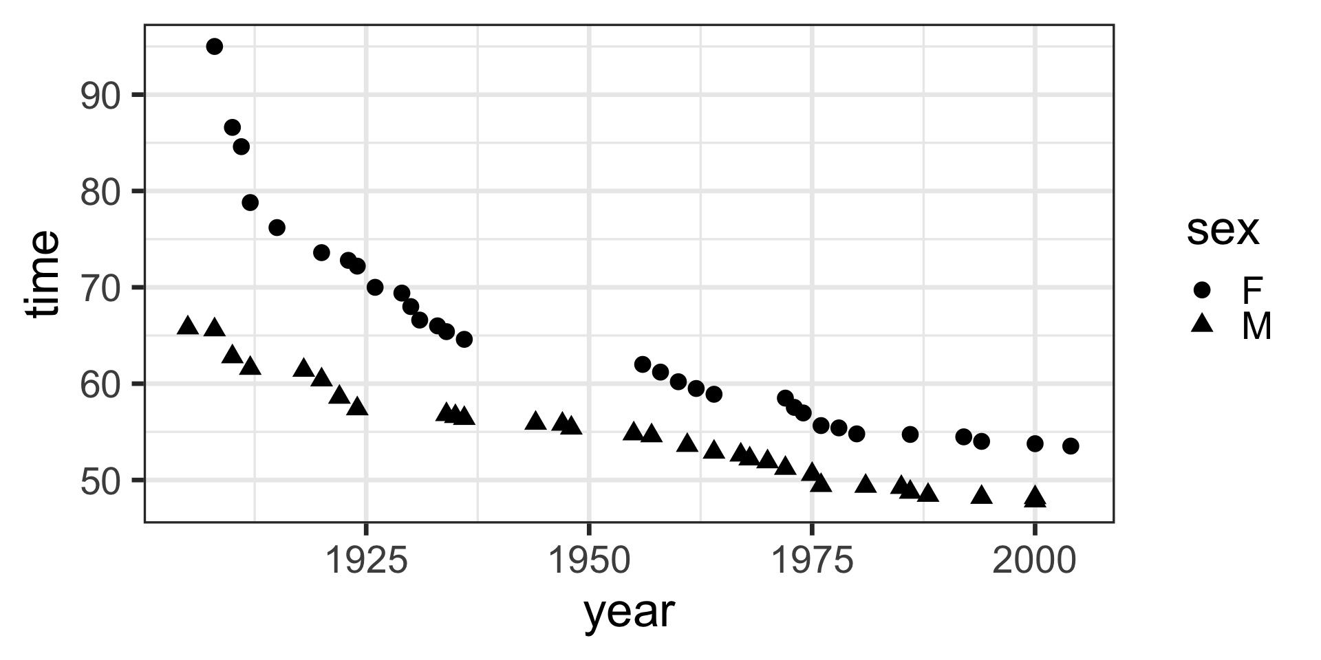
  ggplot(aes(x = year, y = time, shape = sex)) +
  geom_point() +
  geom_line(aes(y = with_predict), color = "blue") +
  theme_bw(base_size = 14)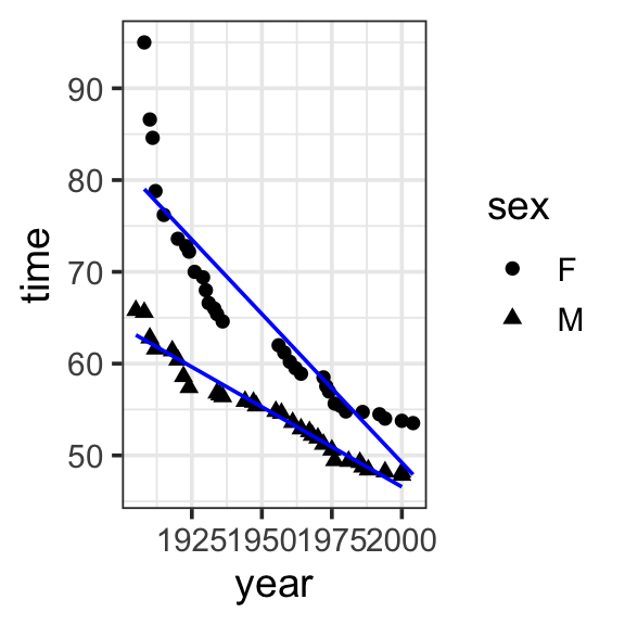

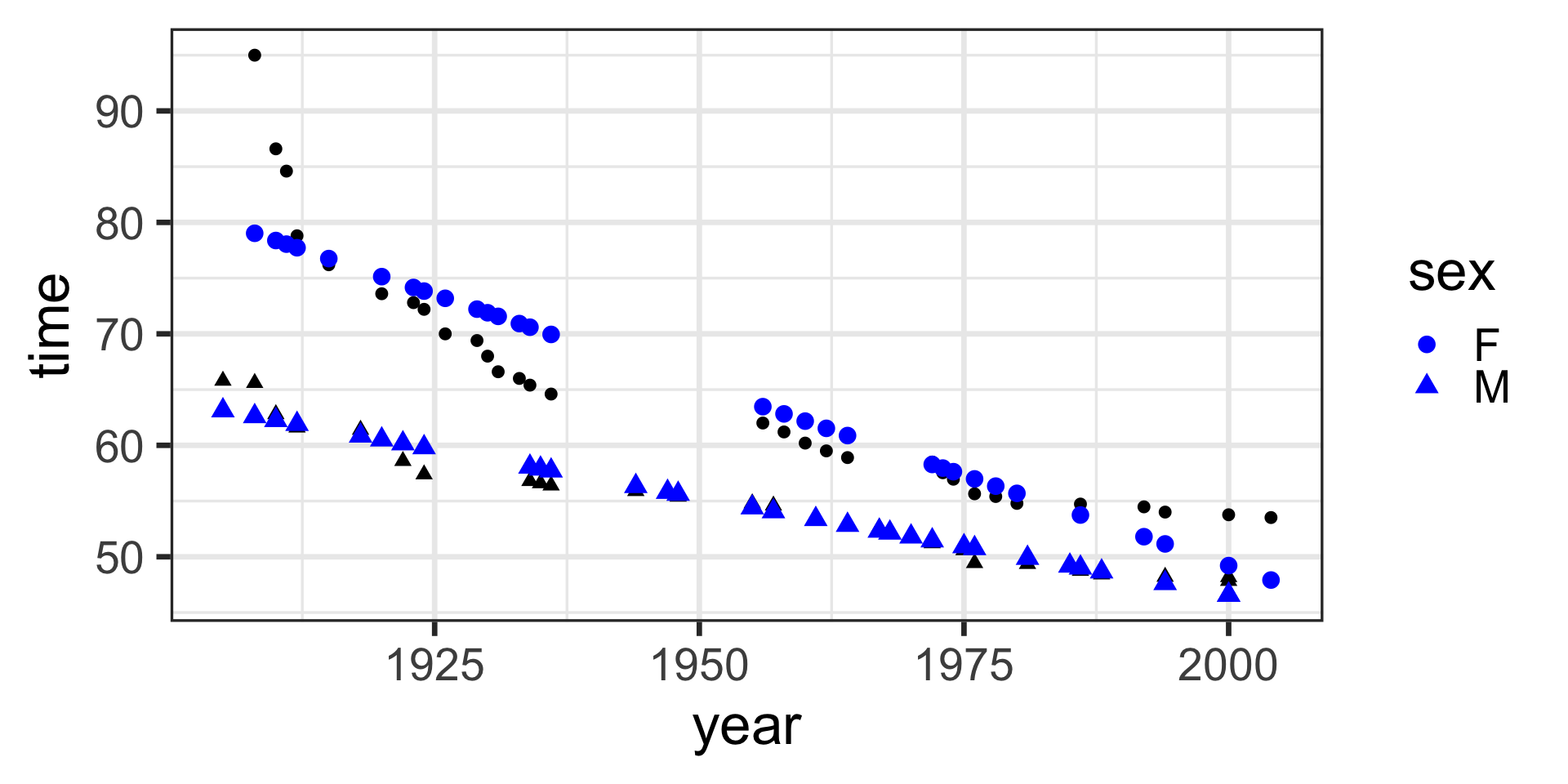
💪In-class exercise

We specified the model including intercept, year, and sex as follows:
$y = w_1\cdot\mathbf{1} + w_2\cdot\mathbf{year} + w_3\cdot\mathbf{sex}$

Fit the model with infer this time. What are the following weights:

$w_1 = $
$w_2 = $
$w_3 = $

Interaction

Plot
Data
Code

Model specification:
$y = w_1\cdot\mathbf{1} + w_2\cdot\mathbf{year} + w_3\cdot\mathbf{sex} + w_4\cdot\mathbf{year\times{sex}}$


Call:
lm(formula = time ~ 1 + year * sex, data = SwimRecords)

Coefficients:
(Intercept)         year         sexM    year:sexM  
   697.3012      -0.3240    -302.4638       0.1499

Fitted model:
\[\begin{align} y = &697.3012 \cdot \mathbf{1} + -0.3240 \cdot \mathbf{year} + -302.4638 \cdot \mathbf{sex}\\ &+ 0.1499 \cdot \mathbf{year\times{sex}} \end{align}\]

year	time	sex	with_predict
1905	65.80	M	63.12106
1908	65.60	M	62.59867
1910	62.80	M	62.25041
1912	61.60	M	61.90215
1918	61.40	M	60.85738
1920	60.40	M	60.50912
1922	58.60	M	60.16086
1924	57.40	M	59.81260
1934	56.80	M	58.07131
1935	56.60	M	57.89718
1936	56.40	M	57.72305
1944	55.90	M	56.33002
1947	55.80	M	55.80763
1948	55.40	M	55.63350
1955	54.80	M	54.41459
1957	54.60	M	54.06634
1961	53.60	M	53.36982
1964	52.90	M	52.84743
1967	52.60	M	52.32504
1968	52.20	M	52.15091
1970	51.90	M	51.80266
1972	51.22	M	51.45440
1975	50.59	M	50.93201
1976	49.44	M	50.75788
1981	49.36	M	49.88723
1985	49.24	M	49.19072
1986	48.74	M	49.01659
1988	48.42	M	48.66833
1994	48.21	M	47.62355
2000	48.18	M	46.57878
2000	47.84	M	46.57878
1908	95.00	F	79.02170
1910	86.60	F	78.37361
1911	84.60	F	78.04956
1912	78.80	F	77.72552
1915	76.20	F	76.75338
1920	73.60	F	75.13315
1923	72.80	F	74.16101
1924	72.20	F	73.83697
1926	70.00	F	73.18887
1929	69.40	F	72.21674
1930	68.00	F	71.89269
1931	66.60	F	71.56864
1933	66.00	F	70.92055
1934	65.40	F	70.59651
1936	64.60	F	69.94842
1956	62.00	F	63.46750
1958	61.20	F	62.81941
1960	60.20	F	62.17131
1962	59.50	F	61.52322
1964	58.90	F	60.87513
1972	58.50	F	58.28276
1973	57.54	F	57.95872
1974	56.96	F	57.63467
1976	55.65	F	56.98658
1978	55.41	F	56.33849
1980	54.79	F	55.69040
1986	54.73	F	53.74612
1992	54.48	F	51.80185
1994	54.01	F	51.15375
2000	53.77	F	49.20948
2004	53.52	F	47.91330

model <- lm(time ~ 1 + year * sex, data = SwimRecords)

SwimRecords_predict <- SwimRecords %>%
  mutate(with_predict= predict(model, SwimRecords))

SwimRecords_predict %>%
  ggplot(aes(x = year, y = time, shape = sex)) +
  geom_point() +
  geom_line(aes(y = with_predict), color = "blue") +
  theme_bw(base_size = 14)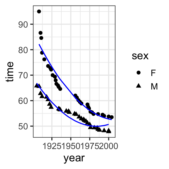

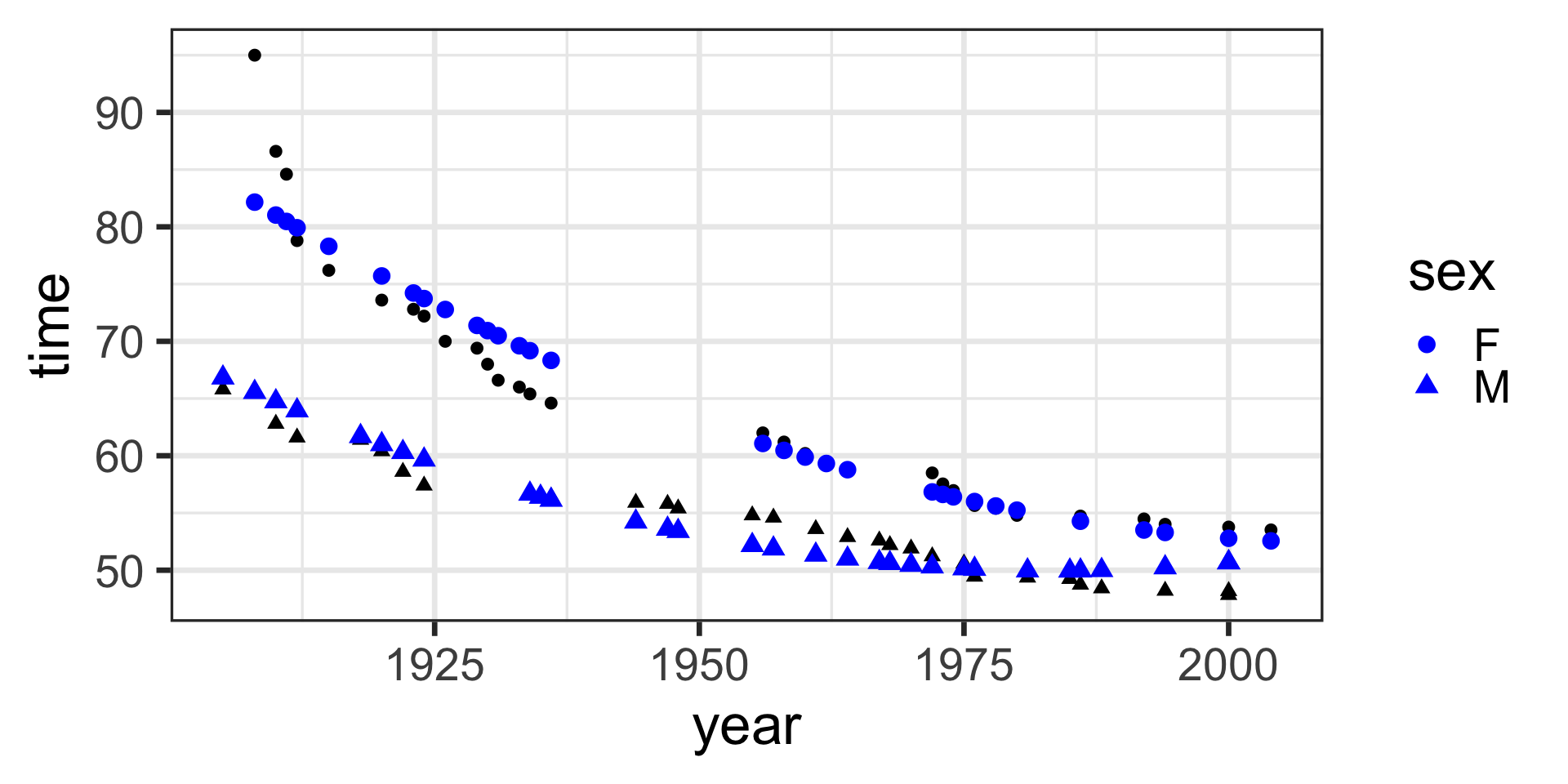
Transformation

Plot
Data
Code

Model specification:
\[\begin{align} y = &w_1\cdot\mathbf{1} + w_2\cdot\mathbf{year} + w_3\cdot\mathbf{sex} \\ &+ w_4\cdot\mathbf{year\times{sex}} +w_5\cdot\mathbf{year}^2 \end{align}\]


Call:
lm(formula = time ~ 1 + year * sex + I(year^2), data = SwimRecords)

Coefficients:
(Intercept)         year         sexM    I(year^2)    year:sexM  
  1.110e+04   -1.098e+01   -3.171e+02    2.729e-03    1.575e-01

Fitted model:
\[\begin{align} y = &11100 \cdot \mathbf{1} + -10.98 \cdot \mathbf{year} + -317.1 \cdot \mathbf{sex}\\ &+ 0.1575 \cdot \mathbf{year\times{sex}} + 0.002729 \cdot \mathbf{year}^2 \end{align}\]

year	time	sex	with_predict
1905	65.80	M	66.81874
1908	65.60	M	65.55576
1910	62.80	M	64.74106
1912	61.60	M	63.94819
1918	61.40	M	61.70057
1920	60.40	M	60.99502
1922	58.60	M	60.31130
1924	57.40	M	59.64941
1934	56.80	M	56.66741
1935	56.60	M	56.39922
1936	56.40	M	56.13650
1944	55.90	M	54.23115
1947	55.80	M	53.60669
1948	55.40	M	53.40946
1955	54.80	M	52.18160
1957	54.60	M	51.87991
1961	53.60	M	51.34200
1964	52.90	M	50.99587
1967	52.60	M	50.69886
1968	52.20	M	50.61078
1970	51.90	M	50.45097
1972	51.22	M	50.31300
1975	50.59	M	50.14697
1976	49.44	M	50.10254
1981	49.36	M	49.96226
1985	49.24	M	49.94827
1986	48.74	M	49.95841
1988	48.42	M	49.99508
1994	48.21	M	50.23605
2000	48.18	M	50.67349
2000	47.84	M	50.67349
1908	95.00	F	82.16082
1910	86.60	F	81.03116
1911	84.60	F	80.47451
1912	78.80	F	79.92332
1915	76.20	F	78.30250
1920	73.60	F	75.71028
1923	72.80	F	74.22044
1924	72.20	F	73.73474
1926	70.00	F	72.77971
1929	69.40	F	71.38810
1930	68.00	F	70.93515
1931	66.60	F	70.48765
1933	66.00	F	69.60903
1934	65.40	F	69.17790
1936	64.60	F	68.33203
1956	62.00	F	61.07389
1958	61.20	F	60.46814
1960	60.20	F	59.88422
1962	59.50	F	59.32213
1964	58.90	F	58.78187
1972	58.50	F	56.83913
1973	57.54	F	56.62085
1974	56.96	F	56.40802
1976	55.65	F	55.99874
1978	55.41	F	55.61129
1980	54.79	F	55.24567
1986	54.73	F	54.27978
1992	54.48	F	53.51036
1994	54.01	F	53.29755
2000	53.77	F	52.79009
2004	53.52	F	52.56093

model <- lm(time ~ 1 + year * sex + I(year^2), data = SwimRecords)

SwimRecords_predict <- SwimRecords %>%
  mutate(with_predict= predict(model, SwimRecords))

SwimRecords_predict %>%
  ggplot(aes(x = year, y = time, shape = sex)) +
  geom_point() +
  geom_line(aes(y = with_predict), color = "blue") +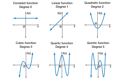
  theme_bw(base_size = 14)

Linearizing nonlinear models

Two common ways:

Expanding the input space with polynomials. Polynomials can capture “bumps” or curves in the data. In this approach, we add terms to the model, like squares or cubes of the original variable.
- $y = w_1 + w_2x + w_3x^2$
Transforming the data involves applying mathematical functions to existing inputs to alter their scale or distributions. Taking the logarithm of a variable compresses its range and reduces skewness in the data (as in the brain size and body weight data).
- both output and input: $log(y) = w_1 + w_2 log(x)$
- just input: $y = w_1 + w_2 log(x)$

Plant heights (polynomials)

poly_plants <- read_csv('https://kschuler.github.io/datasci/assests/csv/polynomial_plants.csv')

Polynomials

Polynomials capture “bumps” or curves in the data, and the number of these bumps depends on the degree of the polynomial. The higher the degree, the more complex the shape the polynomial can represent.

Degree 1 (Linear)

Plot
Data
Code

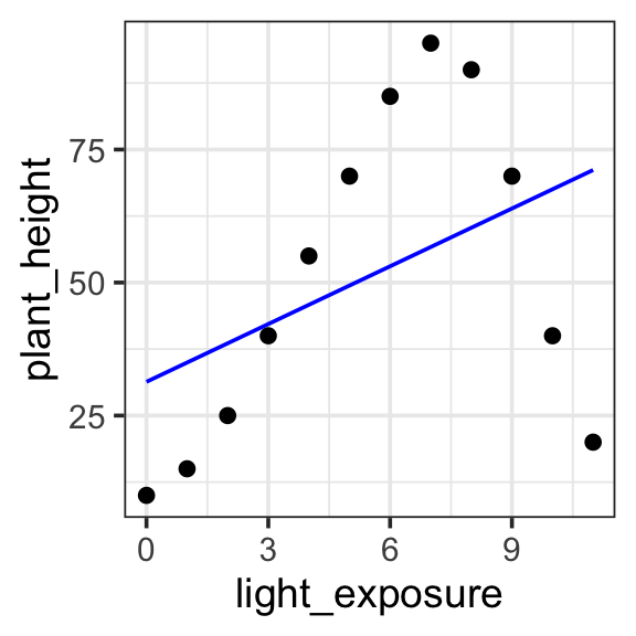
Model specification:
$y = w_1\cdot\mathbf{1} + w_2 \cdot \mathbf{x}$


Call:
lm(formula = plant_height ~ 1 + light_exposure, data = poly_plants)

Coefficients:
   (Intercept)  light_exposure  
        31.346           3.619

Fitted model:
$y = 31.346 \cdot 1 + 3.619 \cdot x$

plant	light_exposure	plant_height	with_formula	with_predict
Sunflower	0	10	31.346	31.34615
Sunflower	1	15	34.965	34.96504
Sunflower	2	25	38.584	38.58392
Rose	3	40	42.203	42.20280
Rose	4	55	45.822	45.82168
Rose	5	70	49.441	49.44056
Cactus	6	85	53.060	53.05944
Cactus	7	95	56.679	56.67832
Cactus	8	90	60.298	60.29720
Orchid	9	70	63.917	63.91608
Orchid	10	40	67.536	67.53496
Orchid	11	20	71.155	71.15385

poly_plants <- read_csv('https://kschuler.github.io/datasci/assests/csv/polynomial_plants.csv')

model <- lm(plant_height ~ 1 + light_exposure, data = poly_plants)

poly_plants <- poly_plants %>%
  mutate(with_formula = 31.346*1 + 3.619*light_exposure) %>%
  mutate(with_predict= predict(model, poly_plants))

poly_plants %>%
  ggplot(aes(x = light_exposure, y = plant_height)) +
  geom_point() +
  geom_line(aes(y = with_predict), color = "blue") +
  theme_bw(base_size = 14)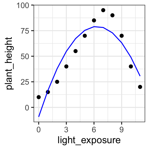

💪In-class exercise

What happens if you specify the model without the intercept term in R? y ~ x instead of y ~ 1 + x?

Try it with the poly_plants data and use ‘lm()’ or ‘infer’ to fit the model you specified. What do you noticed about the weights?

Degree 2 (Quadratic)

Plot
Data
Code

Model specification:
$y = w_1\cdot\mathbf{1} + w_2 \cdot \mathbf{x} + w_3 \cdot \mathbf{x}^2$


Call:
lm(formula = plant_height ~ 1 + light_exposure + I(light_exposure^2), 
    data = poly_plants)

Coefficients:
        (Intercept)       light_exposure  I(light_exposure^2)  
             -9.245               27.973               -2.214

Fitted model:
$y = -9.245 \cdot\mathbf{1} + 27.973 \cdot \mathbf{x} + -2.214 \cdot \mathbf{x}^2$

plant	light_exposure	plant_height	with_predict
Sunflower	0	10	-9.244506
Sunflower	1	15	16.514735
Sunflower	2	25	37.845904
Rose	3	40	54.749001
Rose	4	55	67.224026
Rose	5	70	75.270979
Cactus	6	85	78.889860
Cactus	7	95	78.080669
Cactus	8	90	72.843407
Orchid	9	70	63.178072
Orchid	10	40	49.084665
Orchid	11	20	30.563187


model <- lm(plant_height ~ 1 + light_exposure + I(light_exposure^2), data = poly_plants)

poly_plants <- poly_plants %>%
  mutate(with_predict= predict(model, poly_plants))

poly_plants %>%
  ggplot(aes(x = light_exposure, y = plant_height)) +
  geom_point() +
  geom_line(aes(y = with_predict), color = "blue") +
  theme_bw(base_size = 14)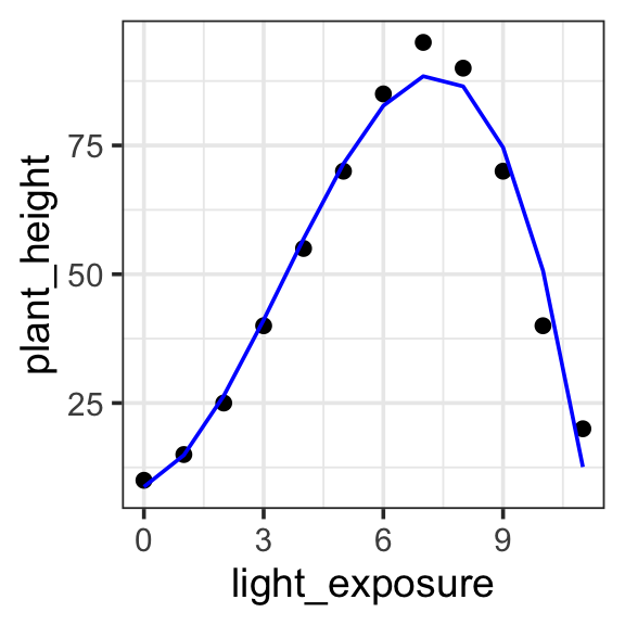

Degree 3 (Cubic)

Plot
Data
Code

Model specification:
$y = w_1\cdot\mathbf{1} + w_2 \cdot \mathbf{x} + w_3 \cdot \mathbf{x}^2 + w_4 \cdot \mathbf{x}^3$


Call:
lm(formula = plant_height ~ 1 + light_exposure + I(light_exposure^2) + 
    I(light_exposure^3), data = poly_plants)

Coefficients:
        (Intercept)       light_exposure  I(light_exposure^2)  
             8.7363               2.7276               3.7796  
I(light_exposure^3)  
            -0.3632

Fitted model:
$y = 8.7363 \cdot \mathbf{1} + 2.7276 \cdot \mathbf{x} + 3.7796 \cdot \mathbf{x}^2 + -0.3632 \cdot \mathbf{x}^3$

plant	light_exposure	plant_height	with_predict
Sunflower	0	10	8.736264
Sunflower	1	15	14.880120
Sunflower	2	25	26.403596
Rose	3	40	41.127206
Rose	4	55	56.871462
Rose	5	70	71.456877
Cactus	6	85	82.703963
Cactus	7	95	88.433233
Cactus	8	90	86.465202
Orchid	9	70	74.620380
Orchid	10	40	50.719281
Orchid	11	20	12.582418

model <- lm(plant_height ~ 1 + light_exposure + I(light_exposure^2) + I(light_exposure^3), data = poly_plants)

poly_plants <- poly_plants %>%
  mutate(with_predict= predict(model, poly_plants))

poly_plants %>%
  ggplot(aes(x = light_exposure, y = plant_height)) +
  geom_point() +
  geom_line(aes(y = with_predict), color = "blue") +
  theme_bw(base_size = 14)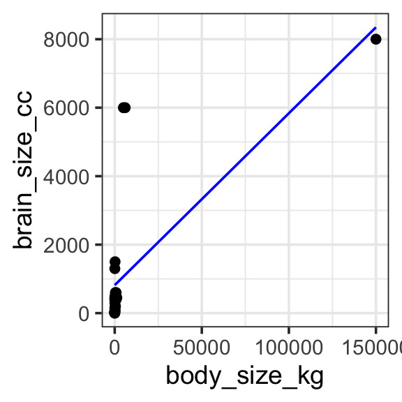

Brain size (log)

brain_data <- read_csv('https://kschuler.github.io/datasci/assests/csv/animal_brain_body_size.csv')

Untransformed

Plot
Data
Code

Model specification:
$y = w_1\cdot\mathbf{1} + w_2\cdot\mathbf{body\_size\_kg}$


Call:
lm(formula = brain_size_cc ~ 1 + body_size_kg, data = brain_data)

Coefficients:
 (Intercept)  body_size_kg  
   816.59014       0.05021

Fitted model:
$y = 816.59014 \cdot\mathbf{1} + 0.05021 \cdot\mathbf{body\_size\_kg}$

Species	brain_size_cc	body_size_kg	with_predict
Mouse	0.4	2.0e-02	816.5911
Rat	2.0	2.5e-01	816.6027
Rabbit	12.0	1.5e+00	816.6655
Cat	25.0	4.5e+00	816.8161
Dog	50.0	1.0e+01	817.0923
Sheep	150.0	7.0e+01	820.1049
Pig	300.0	1.0e+02	821.6113
Goat	450.0	5.0e+01	819.1007
Gorilla	500.0	1.8e+02	825.6282
Horse	600.0	4.0e+02	836.6747
Human	1300.0	7.0e+01	820.1049
Chimpanzee	400.0	6.0e+01	819.6028
Dolphin	1500.0	2.0e+02	826.6324
Whale (Orca)	6000.0	5.0e+03	1067.6469
Elephant	6000.0	6.0e+03	1117.8583
Blue Whale	8000.0	1.5e+05	8348.2943
Giraffe	600.0	8.0e+02	856.7592
Rhinoceros	450.0	1.2e+03	876.8438
Walrus	400.0	8.0e+02	856.7592
Tiger	90.0	2.2e+02	827.6366
Kangaroo	50.0	6.0e+01	819.6028
Crocodile	200.0	4.0e+02	836.6747
Penguin	20.0	3.0e+01	818.0965

brain_data <- read_csv('https://kschuler.github.io/datasci/assests/csv/animal_brain_body_size.csv') %>%
  rename(brain_size_cc = `Brain Size (cc)`, body_size_kg = `Body Size (kg)`)

model <- lm(brain_size_cc ~ 1 + body_size_kg, data = brain_data)

brain_data <- brain_data %>%
  mutate(with_predict= predict(model, brain_data))

brain_data %>%
  ggplot(aes(x = body_size_kg, y = brain_size_cc)) +
  geom_point() +
  geom_line(aes(y = with_predict), color = "blue") +
  theme_bw(base_size = 14)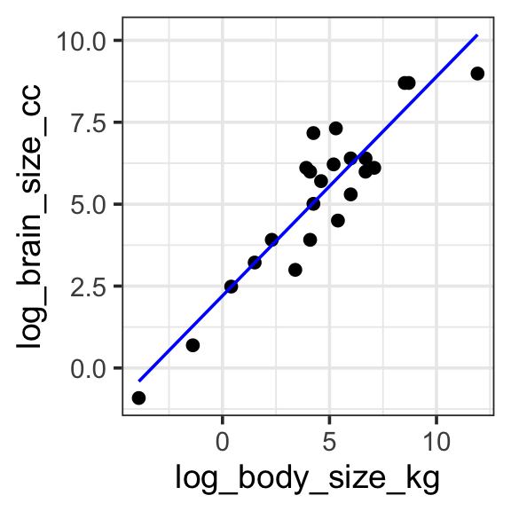

Log transformed

Plot
Data
Code

Model specification:
$log(y) = w_1\cdot\mathbf{1} + w_2 \cdot log(\mathbf{body\_size\_kg})$


Call:
lm(formula = log(brain_size_cc) ~ 1 + log(body_size_kg), data = brain_data)

Coefficients:
      (Intercept)  log(body_size_kg)  
           2.2042             0.6687

Fitted model:
$log(y) = 2.2042\cdot\mathbf{1} + 0.6687 \cdot log(\mathbf{body\_size\_kg})$

Species	brain_size_cc	body_size_kg	log_brain_size_cc	log_body_size_kg	with_predict
Mouse	0.4	2.0e-02	-0.9162907	-3.9120230	-0.4116321
Rat	2.0	2.5e-01	0.6931472	-1.3862944	1.2772249
Rabbit	12.0	1.5e+00	2.4849066	0.4054651	2.4753051
Cat	25.0	4.5e+00	3.2188758	1.5040774	3.2099046
Dog	50.0	1.0e+01	3.9120230	2.3025851	3.7438358
Sheep	150.0	7.0e+01	5.0106353	4.2484952	5.0449906
Pig	300.0	1.0e+02	5.7037825	4.6051702	5.2834853
Goat	450.0	5.0e+01	6.1092476	3.9120230	4.8200046
Gorilla	500.0	1.8e+02	6.2146081	5.1929569	5.6765155
Horse	600.0	4.0e+02	6.3969297	5.9914645	6.2104467
Human	1300.0	7.0e+01	7.1701195	4.2484952	5.0449906
Chimpanzee	400.0	6.0e+01	5.9914645	4.0943446	4.9419160
Dolphin	1500.0	2.0e+02	7.3132204	5.2983174	5.7469660
Whale (Orca)	6000.0	5.0e+03	8.6995147	8.5171932	7.8993037
Elephant	6000.0	6.0e+03	8.6995147	8.6995147	8.0212150
Blue Whale	8000.0	1.5e+05	8.9871968	11.9183906	10.1735527
Giraffe	600.0	8.0e+02	6.3969297	6.6846117	6.6739274
Rhinoceros	450.0	1.2e+03	6.1092476	7.0900768	6.9450462
Walrus	400.0	8.0e+02	5.9914645	6.6846117	6.6739274
Tiger	90.0	2.2e+02	4.4998097	5.3936275	5.8106962
Kangaroo	50.0	6.0e+01	3.9120230	4.0943446	4.9419160
Crocodile	200.0	4.0e+02	5.2983174	5.9914645	6.2104467
Penguin	20.0	3.0e+01	2.9957323	3.4011974	4.4784353

model <- lm(log(brain_size_cc) ~ 1 + log(body_size_kg), data = brain_data)

brain_data <- brain_data %>%
  mutate(
    log_brain_size_cc = log(brain_size_cc), 
    log_body_size_kg = log(body_size_kg)
  ) %>%
  mutate(with_predict= predict(model, brain_data))

brain_data %>%
  ggplot(aes(x = log_body_size_kg, y = log_brain_size_cc)) +
  geom_point() +
  geom_line(aes(y = with_predict), color = "blue") +
  theme_bw(base_size = 14)

Model Specification

Tuesday

Announcements

You are here

Data science with R

Stats & Model building

More advanced

Review

Exploring relationships

Is there a relationship?

Yes, a linear relationship

Quantify with correlation

Computing correlation in R

Correlation uncertainty

💪 In-class Exercise

Hypothesis testing our correlation

Hypothesis testing our correlation

Model building

Correlation is model building

Correlation is model building

How do we get \(r = 0.48\) ?

Correlation is the slope of the model

Model building overview

Types of models

💪 In-class Exercise

Supervised learning

Supervised learning

Supervised learning

Types of models

Regression v classification

Types of models

Linear models

Linear model equation

Types of models

Nonlinear models

💪 In-class Exercise

Model specification

Model specification

Specifying the functional form

🥸 Aliases of \(y=\sum_{i=1}^{n}w_ix_i\)

Specify our first model

💪 In class exercise

Swim Records

Specify a model for SwimRecords

💪 In class exercise

Response variable \(y\)

Explanatory variable(s) \(x_i\)

Functional form

Model terms

Intercept

Main

Interaction

Transformation

THursday

Model building overview

Types of models

Regression v classification

Linear v Nonlinear models

Model specification

“Toy” data

Explore the data

💪In-class exercise

Specify, fit, plot model

Swim records

One input

💪In-class exercise

Two inputs

Three inputs

💪In-class exercise

Interaction

Transformation

Linearizing nonlinear models

Plant heights (polynomials)

Polynomials

Degree 1 (Linear)

💪In-class exercise

Degree 2 (Quadratic)

Degree 3 (Cubic)

Brain size (log)

Untransformed

You are `here`

Specify a model for `SwimRecords`