R basics

Data Science for Studying Language and the Mind

Katie Schuler

2024-08-28

Syllabus

Follow along on the syllabus!

Paperwork

When you arrive, complete this anonymous form: Who’s in class
You can also join the waitlist if you are not enrolled

Announcements

The course is full and the room is full
Ways to join:
1. Watch for an opening (highest odds of getting in)
2. Add your name to our waitlist

Course description

Data Sci for Lang & Mind is an entry-level course designed to teach basic principles of statistics and data science to students with little or no background in statistics or computer science. Students will learn to identify patterns in data using visualizations and descriptive statistics; make predictions from data using machine learning and optimization; and quantify the certainty of their predictions using statistical models. This course aims to help students build a foundation of critical thinking and computational skills that will allow them to work with data in all fields related to the study of the mind (e.g. linguistics, psychology, philosophy, cognitive science, neuroscience).

Prerequisites

There are no prerequisites beyond high school algebra. No prior programming or statistics experience is necessary, though you will still enjoy this course if you already have a little. Students who have taken several computer science or statistics classes should look for a more advanced course.

Teaching team

Instructor: Dr. Katie Schuler (she/her)

TAs:

Brittany Zykoski
Mingyang Bian

About me, your instructor (Katie)

You can call me Professor Schuler or Katie, whichever makes you more comfortable
I live in Mt Airy with my husband and two kids (Dory, 2 and Joan, 6)
At Penn I also have a research lab, the Child Language Lab and am on the Natural Science and Math Panel (a group focused on improving inclusive teaching in STEM at Penn).
I’m a first-generation college student from Western NY. I worked 40 hours a week to put myself through college; I am still paying off my student loans.

My assumptions about you

You are an honest, kind, and hardworking person who wants to do well in and enjoy this class

You are very busy, and will sometimes have to prioritize other things above this class.

Course overview

Data science

Data science is about making decisions based on incomplete information.

This concept is not new. Brains were built for doing this!

But we have new tools and lots more data!

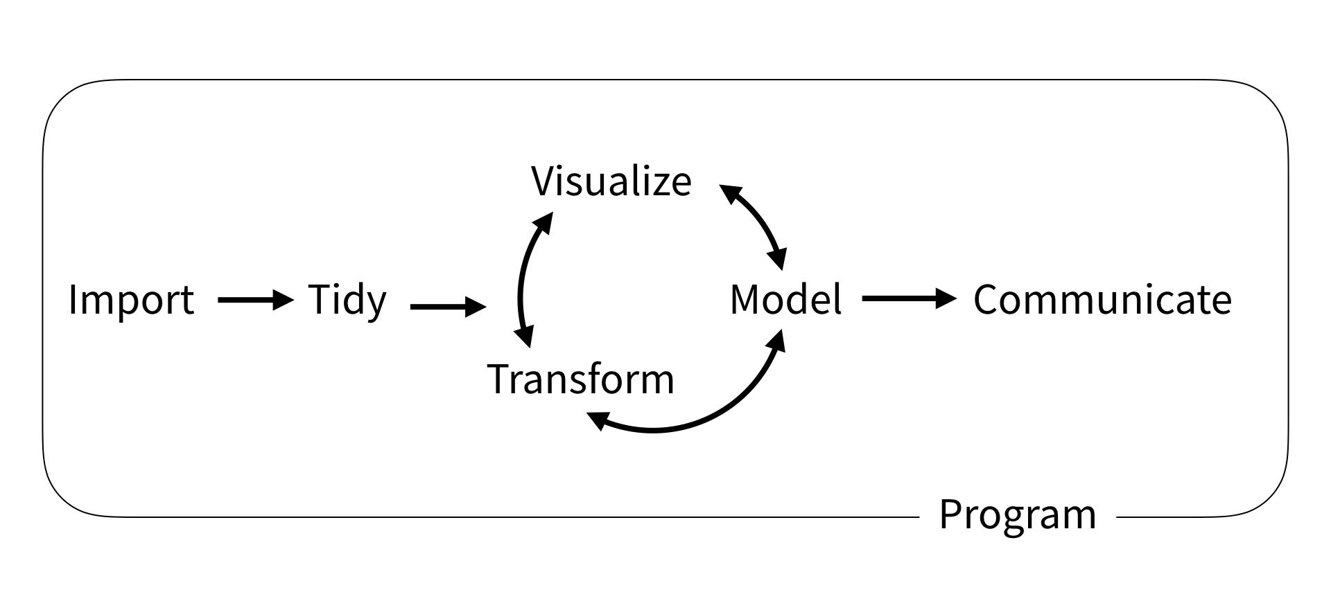
Figure 2: from https://web-assets.domo.com/miyagi/images/product/product-feature-22-data-never-sleeps-10.png

Data science workflow

The folks who wrote R for Data Science proposed the following data science workflow:

Overview of course

We will spend the first few weeks getting comfortable programming in R, including some useful skills for data science:

R basics
Data visualization
Data wrangling (import, tidy, and transform)

Overview of course

Then, we will spend the next several weeks building a foundation in basic statistics and model building:

Sampling distribution
Hypothesis testing
Model specification
Model fitting
Model evaluation (accuracy and reliability)

Overview of course

Finally if we have time we will cover a selection of more advanced topics that are often applied in language and mind fields, with a focus on basic understanding:

Feature engineering
Classification
Mixed-effect models

Syllabus, briefly

Each week will include two lectures and a lab:

Lectures are on Tuesdays and Thursdays at 12pm and will be a mix of conceptual overviews and R tutorials. It is a good idea to bring your laptop so you can follow along and try stuff in R!
Labs are on Thursday or Friday and will consist of (ungraded) practice problems and concept review with TAs. You may attend any lab section that works for your schedule. Lab attendance is required

Syllabus, briefly

There are 10 graded assessments:

8 Problem sets (20%) in which you will be asked to apply your newly aquired R programming skills.
2 Midterm exams (60%) in which you will be tested on your understanding of lecture concepts.

And 20% is lab attendance.

Syllabus, briefly

There are a few policies to take note of:

Missed exams cannot be made up except in cases of genuine conflict or emergency (documentation and course action notice required). You may take the optional final exam to replace a missed or low scoring exam.
You may request an extension on any problem set of up to 3 days. But extensions beyond 3 days will not be granted (because delying solutions will negative impact other students).
You may submit any missed quiz or problem set by the end of the semester for half-credit (50%), even after solutions are posted.
We will drop your lowest pset grade, and you can miss up to 2 labs without penalty

Resources

In addition to our course website, we will use the following:

google colab (r kernel) - for computing
canvas- for posting grades
gradescope - for submitting problem sets
ed discussion - for announcements and questions

Wellness resources

Please consider using these Penn resources this semester:

Weingarten Center for academic support and tutoring.
Wellness at Penn for health and wellbeing.

Why R?

With many programming languages available for data science (e.g. R, Python, Julia, MATLAB), why use R?

Built for stats, specifically
Makes nice visualizations
Lots of people are doing it, especially in academia
Easier for beginners to understand
Free and open source (though so are Python and Julia, MATLAB costs $)

Many ways to use R

R Studio
Jupyter
VS Code
and even simply the command line/terminal

Google Colab

Google Colab is a cloud-based Jupyter notebook that allows you to write, execute, and share code like a google doc.
We use Google Colab because it’s simple and accessible to everyone. You can start programming right away, no setup required!

Secretly, R!

Google Colab officially supports Python, but secretly supports R (and Julia, too!)

Update 2024: Google Colab now officially supports R!
Update 2025: Google Colab officially supports Julia!
colab (r kernel)

Let’s try it!

Google colab demo

Open a new R notebook:

colab (r kernel) - use this link to start a new R notebook
File > New notebook and then Runtime > Change runtime type to R

Cell types:

+ Code - write and execute code
+ Text - write text blocks in markdown

Frequently used keyboard shortcuts:

Cmd/Ctrl+S - save
Cmd/Ctrl+Enter - run focused cell
Cmd/Ctrl+Shift+A - select all cells
Cmd/Ctrl+/ - comment/uncomment selection
Cmd/Ctrl+] - increase indent
Cmd/Ctrl+[ - decrease indent

You are `here`

Data science with R

R basics
Data visualization
Data wrangling

Stats & Model buidling

Sampling distribution
Hypothesis testing
Model specification
Model fitting
Model evaluation

More advanced

Feature Engineering
Classification
Mixed-effect models

R Basics

We begin by defining some basic concepts:

Basic concepts

Expressions: fundamental building blocks of programming
Objects: allow us to store stuff, created with assignment operator
Names: names w give objects must be letters, numbers, ., or _
Attributes: allow us to attach arbitrary metadata to objects
Functions: take some input, perform some computation, and return some output
Environment: collection of all objects we defined in current R session
Packages: collections of functions, data, and documentation bundled together in R
Comments: notes you leave for yourself, not evaluated
Messages: notes R leaves for you (FYI, warning, error)

Expressions

Expressions are combinations of values, variables, operators, and functions that can be evaluated to produce a result. Expressions can be as simple as a single value or more complex involving calculations, comparisons, and function calls. They are the fundamental building blocks of programming.
- 10 - a simple value expression that evaluates to 10.
- x <- 10 - an expression that assigns the value of 10 to x.
- x + 10 - an expression that adds the value of x to 10.
- a <- x + 10 - an expression that adds the value of x to 10 and assigns the result to the variable a

Important functions

Objects

str(x) - returns summary of object’s structure
typeof(x) - returns object’s data type
length(x) - returns object’s length
attributes(x) - returns list of object’s attributes

Important functions

Environment

ls() - list all variables in environment
rm(x) - remove x variable from environment
rm(list = ls()) - remove all variables from environment

Thursday Aug 28

Thursday’s class started here.

Important function

Packages

install.packages() to install packages
library() to load package into current R session.
data() to load data from package into environment
sessionInfo() - version info, packages for current R session

Important functions

Help

?mean - get help with a function
help('mean') - search help files for word or phrase
help(package='tidyverse') - find help for a package

Vectors

are fundamental data structures in R. There are two types:

atomic vectors - elements of the same data type
lists - elements refer to any object

Atomic vectors

Atomic vectors can be one of six data types:

`typeof(x)`	examples
double	3, 3.32
integer	1L, 144L
character	“hello”, ‘hello, world!’
logical	TRUE, F

atomic because they must contain only one type

Atomic vectors

double

typeof(3.34)

[1] "double"

integer

typeof(3L)

[1] "integer"

character

typeof('hello, world!')

[1] "character"

logical

typeof(TRUE)

[1] "logical"

Create a vector

with c() for concatenate

c(2,4,6)

[1] 2 4 6

c("hello", "world", "!")

[1] "hello" "world" "!"

c(T, F, T)

[1]  TRUE FALSE  TRUE

c("hello", c(2, 3))

[1] "hello" "2"     "3"

Create a vector

with sequences seq() or repetitions rep()

# sequence of integers have a special shorthand
6:10

[1]  6  7  8  9 10

# sequence from, to, by 
seq(from=3, to=5, by=0.5)

[1] 3.0 3.5 4.0 4.5 5.0

# rep(x, times = 1, each = 1)
rep(c(1,0), times = 4)

[1] 1 0 1 0 1 0 1 0

# rep(x, times = 1, each = 1)
rep(c(1,0), each = 4)

[1] 1 1 1 1 0 0 0 0

Check data type

with typeof(x) - returns the type of vector x

typeof(3)

[1] "double"

typeof(3L)

[1] "integer"

typeof("three")

[1] "character"

typeof(TRUE)

[1] "logical"

Check data type

with is.*(x) - returns TRUE if x has type *

is.double(3)

[1] TRUE

is.integer(3L)

[1] TRUE

is.character("three")

[1] TRUE

is.logical(TRUE)

[1] TRUE

Coercion, implicit

If you try to include elements of different types, R will coerce them into the same type without warning (implicit coercion)

x <- c(1, 2, "three", 4, 5 )
x

[1] "1"     "2"     "three" "4"     "5"

typeof(x)

[1] "character"

Coercion, explicit

You can also use explict coercion to change a vector to another data type with as.*()

x <- c(1, 0 , 1, 0)
as.logical(x)

[1]  TRUE FALSE  TRUE FALSE

More complex structures

Some more complex data structures are built from atomic vectors by adding attributes:

Structure	Description
`matrix`	vector with `dim` attribute representing 2 dimensions
`array`	vector with `dim` attribute representing n dimensions
`data.frame`	a named list of vectors (of equal length) with attributes for `names` (column names), `row.names`, and `class="data.frame"`

Create more complex structures

matrix

matrix(0, nrow=2, ncol=3)

     [,1] [,2] [,3]
[1,]    0    0    0
[2,]    0    0    0

data.frame

data.frame(x=c(1,2,3), y=c('a','b','c'))

  x y
1 1 a
2 2 b
3 3 c

array

array(0, dim=c(2,3,2))

, , 1

     [,1] [,2] [,3]
[1,]    0    0    0
[2,]    0    0    0

, , 2

     [,1] [,2] [,3]
[1,]    0    0    0
[2,]    0    0    0

Operations

Basic math operators

Operator	Operation
`()`	Parentheses
`^`	Exponent
`*`	Multiply
`/`	Divide
`+`	Add
`-`	Subtract

Basic math operations

follow the order of operations you expect (PEMDAS)

# multiplication takes precedence
2 + 3 * 10

[1] 32

# we can use paratheses to be explicit
(2 + 3) * 10

[1] 50

Comparison operators

Operator	Comparison
`x < y`	less than
`x > y`	greater than
`x <= y`	less than or equal to
`x >= y`	greater than or equal to
`x != y`	not equal to
`x == y`	equal to

Comparison operators

x <- 2
y <- 3

x < y

[1] TRUE

x > y

[1] FALSE

x != y

[1] TRUE

x == y

[1] FALSE

Logical operators

Operator	Operation
`x \| y`	or
`x & y`	and
`!x`	not
`any()`	true if any element meets condition
`all()`	true if all elements meet condition
`%in%`	true if any element is in following vector

Logical operators

x <- TRUE
y <- FALSE

x | y

[1] TRUE

x & y

[1] FALSE

!x

[1] FALSE

any(c(x,y))

[1] TRUE

all(c(x,y))

[1] FALSE

Operations are vectorized

Almost all operations (and many functions) are vectorized

math

c(1, 2, 3) + c(4, 5, 6)

[1] 5 7 9

c(1, 2, 3) / c(4, 5, 6)

[1] 0.25 0.40 0.50

c(1, 2, 3) * 10

[1] 10 20 30

c(1, 2, 30) > 10

[1] FALSE FALSE  TRUE

logical

x <- c(TRUE, FALSE, FALSE)
y <- c(TRUE, TRUE, FALSE)
z <- TRUE

x | y

[1]  TRUE  TRUE FALSE

x & y

[1]  TRUE FALSE FALSE

x | z

[1] TRUE TRUE TRUE

x & z

[1]  TRUE FALSE FALSE

Operator coercion

Operators and functions will also coerce values when needed (and without warning)

5.6 + 2L

[1] 7.6

10 + FALSE

[1] 10

log(1)

[1] 0

log(TRUE)

[1] 0

Subsetting

Subsetting is a natural complement to str(). While str() shows you all the pieces of any object (its structure), subsetting allows you to pull out the pieces that you’re interested in. ~ Hadley Wickham, Advanced R

str()

x <- c("hello", "world", "!")
str(x)

 chr [1:3] "hello" "world" "!"

y <- c(1, 2, 3, 4, 5)
str(y)

 num [1:5] 1 2 3 4 5

Subsetting

There are three operators for subsetting objects:

[ - subsets (one or more) elements
[[ and $ - extracts a single element

Subset multiple elements with `[`

Code	Returns
`x[c(1,2)]`	positive integers select elements at specified indexes
`x[-c(1,2)]`	negative integers select all but elements at specified indexes
`x[c("x", "y")]`	select elements by name, if elements are named
`x[]`	nothing returns the original object
`x[0]`	zero returns a zero-length vector
`x[c(TRUE, TRUE)]`	select elements where corresponding logical value is TRUE

Subset multiple elements with `[`

atomic vector

x <- c("hello", "world", "1")

x[c(1,2)]

[1] "hello" "world"

x[-c(1,2)]

[1] "1"

x[]

[1] "hello" "world" "1"

data.frame

y <- data.frame(
        this = c(1, 2,3), 
        that = c("a", "b", "c"),
        theother = c(4, 5, 6)
        )

y[c(1,2)]

  this that
1    1    a
2    2    b
3    3    c

y[-c(1,2)]

y[c("this")]

3 ways to extract a single element

Code	Returns
`[[2]]`	a single positive integer (index)
`[['name']]`	a single string
`x$name`	the `$` operator is a useful shorthand for `[['name']]`

3 ways to extract a single element

atomic vector

x <- c("hello", "world", "1")

x[[1]]

[1] "hello"

x[[2]]

[1] "world"

x[[3]]

[1] "1"

data.frame

y <- data.frame(
        this = c(1, 2,3), 
        that = c("a", "b", "c"),
        theother = c(4, 5, 6)
        )

y[[1]]

[1] 1 2 3

y[["that"]]

[1] "a" "b" "c"

y$that

[1] "a" "b" "c"

R has many built-in functions

x <- c(1, -2, 3)

Some are vectorized

log(x)

[1] 0.000000      NaN 1.098612

abs(x)

[1] 1 2 3

round(x, 2)

[1]  1 -2  3

Some are not

mean(x)

[1] 0.6666667

max(x)

[1] 3

min(x)

[1] -2

Missing values

NA

used to represent missing or unknown elements in vectors
Note that NA is contageous: expressions including NA usually return NA
Check for NA values with is.na()

x <- c(1, NA, 3)
is.na(x)

[1] FALSE  TRUE FALSE

length(x)

[1] 3

mean(x)

[1] NA

NULL

used to represent an empty or absent vector of arbitrary type
NULL is its own special type and always has length zero and NULL attributes
Check for NULL values with is.null()

x <- c()
is.null(x)

[1] TRUE

length(x)

[1] 0

mean(x)

[1] NA

Programming

functions

are reusable pieces of code that take some input, perform some task or computation, and return an output

function(inputs){
    # do something
    return(output)
}

control flow

refers to managing the order in which expressions are executed in a program

if…else - if something is true, do this; otherwise do that
for loops - repeat code a specific number of times
while loops - repeat code as long as certain conditions are true
break - exit a loop early
next - skip to next iteration in a loop

Subsetting quirks

If we have time

Notes on `[` with higher dim objects

m <- matrix(1:6, nrow=2, ncol=3)
m

     [,1] [,2] [,3]
[1,]    1    3    5
[2,]    2    4    6

# separate dimensions by comma 
m[1, 2]

[1] 3

# omitted dim return all from that dim 
m[2, ]

[1] 2 4 6

m[ , 2]

[1] 3 4

Notes on `[[` and `$`:

both [[ and [ work for vectors; use [[

x <- c(1, -2, 3)
x[[1]]

[1] 1

x[1]

[1] 1

$ does partial matching without warning

df <- data.frame(
        this = c(1, 2,3), 
        that = c("a", "b", "c"),
        theother = c(4, 5, 6)
        )

df[['theo']]

NULL

df$theo

[1] 4 5 6

Questions?

Have a great weekend!

R basics

Syllabus

Paperwork

Announcements

Course description

Prerequisites

Teaching team

About me, your instructor (Katie)

My assumptions about you

Course overview

Data science

But we have new tools and lots more data!

Data science workflow

Overview of course

Overview of course

Overview of course

Syllabus, briefly

Syllabus, briefly

Syllabus, briefly

Resources

Wellness resources

Why R?

Many ways to use R

Google Colab

Secretly, R!

Let’s try it!

Open a new R notebook:

Cell types:

Left sidebar:

Frequently used menu options:

Frequently used keyboard shortcuts:

You are here

Data science with R

Stats & Model buidling

More advanced

R Basics

Basic concepts

Expressions

Important functions

Objects

Important functions

Environment

Thursday Aug 28

Important function

Packages

Important functions

Help

Vectors

Vectors

Atomic vectors

Atomic vectors

Create a vector

Create a vector

Check data type

Check data type

Coercion, implicit

Coercion, explicit

More complex structures

More complex structures

Create more complex structures

Operations

Basic math operators

Basic math operations

Comparison operators

Comparison operators

Logical operators

Logical operators

Operations are vectorized

Operator coercion

Subsetting

Subsetting

Subset multiple elements with [

Subset multiple elements with [

3 ways to extract a single element

3 ways to extract a single element

R has many built-in functions

Missing values

Programming

Subsetting quirks

Notes on [ with higher dim objects

You are `here`

Subset multiple elements with `[`

Subset multiple elements with `[`

Notes on `[` with higher dim objects

Notes on `[[` and `$`: