Sampling Distribution

Data Science for Studying Language and the Mind

Katie Schuler

2025-09-16

Announcements

You are here

Data science with R

• R basics
• Data visualization
• Data wrangling

Stats & Model building

• Sampling distribution
• Hypothesis testing
• Model specification
• Model fitting
• Model evaluation

More advanced

• Feature engineering
• Classification
• Mixed-effect models

Data science workflow

Data Science Workflow by R4DS

Attribution

Inspired by a MATLAB course Katie took by Kendrick Kay

Data

Simulated from Ritchie et al 2018:

Sex Differences in the Adult Human Brain: Evidence from 5216 UK Biobank Participants

Descriptive statistics

Dataset

Suppose we measure a single quantity: brain volume of human adults (in cubic centemeters)

# A tibble: 10 × 1
   volume
    <dbl>
 1  1193.
 2  1150.
 3  1243.
 4  1207.
 5  1236.
 6  1292.
 7  1201.
 8  1259.
 9  1157.
10  1169.

Rows: 5,216
Columns: 1
$ volume <dbl> 1193.283, 1150.383, 1242.702, 1206.808, 1235.955, 1292.399, 120…

Exploring a simple dataset

Each tick mark is one data point: one participant’s brain volume

Visualize the distribution

Visualize the distribution of the data with a histogram

Measure of central tendency

Summarize the data with a single value: mean, a measure of where a central or typical value might fall

Measure of central tendency

Summarize the data with a single value: mean, a measure of where a central or typical value might fall

Measure of variability

Summarize the spread of the data with standard deviation

Measure of variability

Summarize the spread of the data with standard deviation

Parametric statistics

Mean and sd are parametric summary statistics. They are given by the following equations:

\(mean(x) = \bar{x} = \frac{\sum_{i=i}^{n} x_{i}}{n}\)

sd(\(x\)) = \(\sqrt{\frac{\sum_{i=1}^n (x_i - \bar{x})^2}{n-1}}\)

\(mean(x) = \bar{x} = \frac{\sum_{i=i}^{n} x_{i}}{n}\)

sd(\(x\)) = \(\sqrt{\frac{\sum_{i=1}^n (x_i - \bar{x})^2}{n-1}}\)

Nonparametric statistics

• Mean and sd are a good summary of the data when the distribution is normal (gaussian)
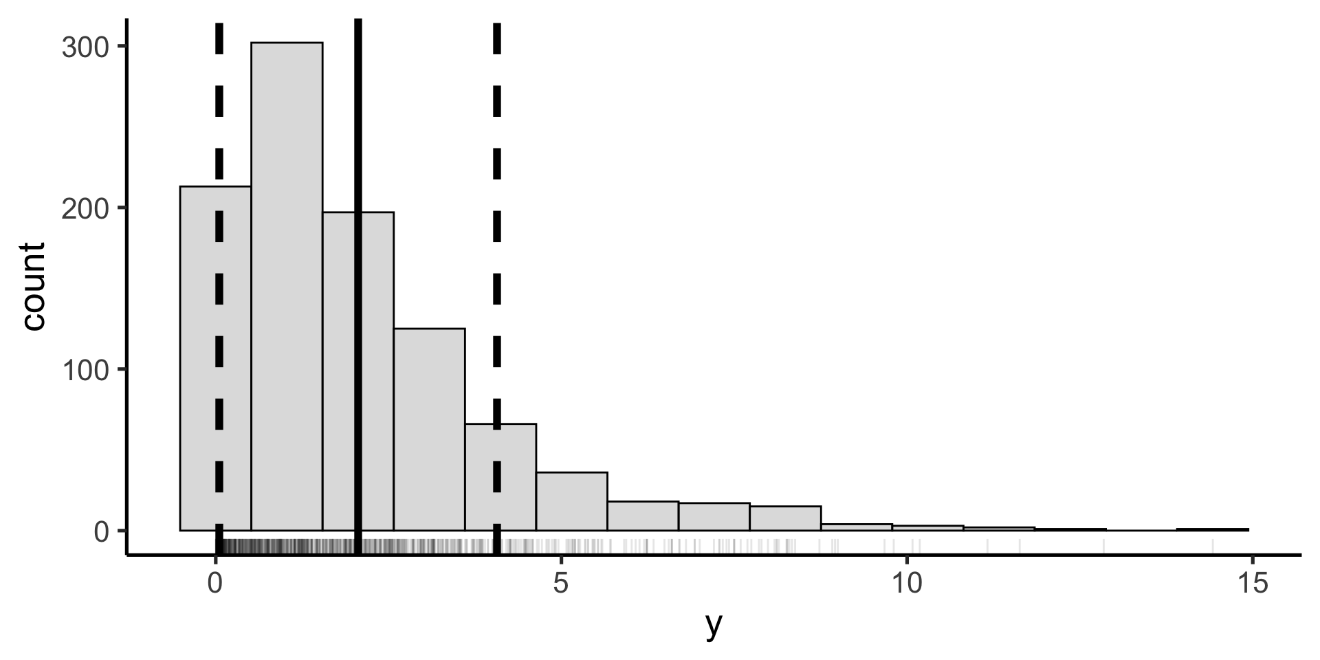
• But suppose our distribution is not normal.

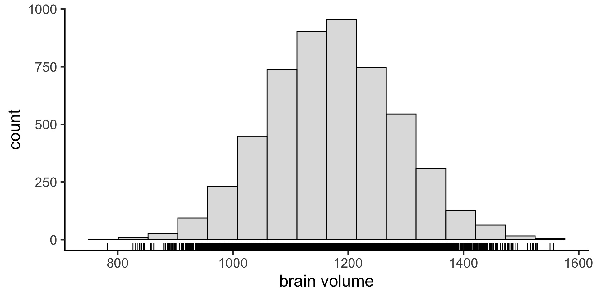
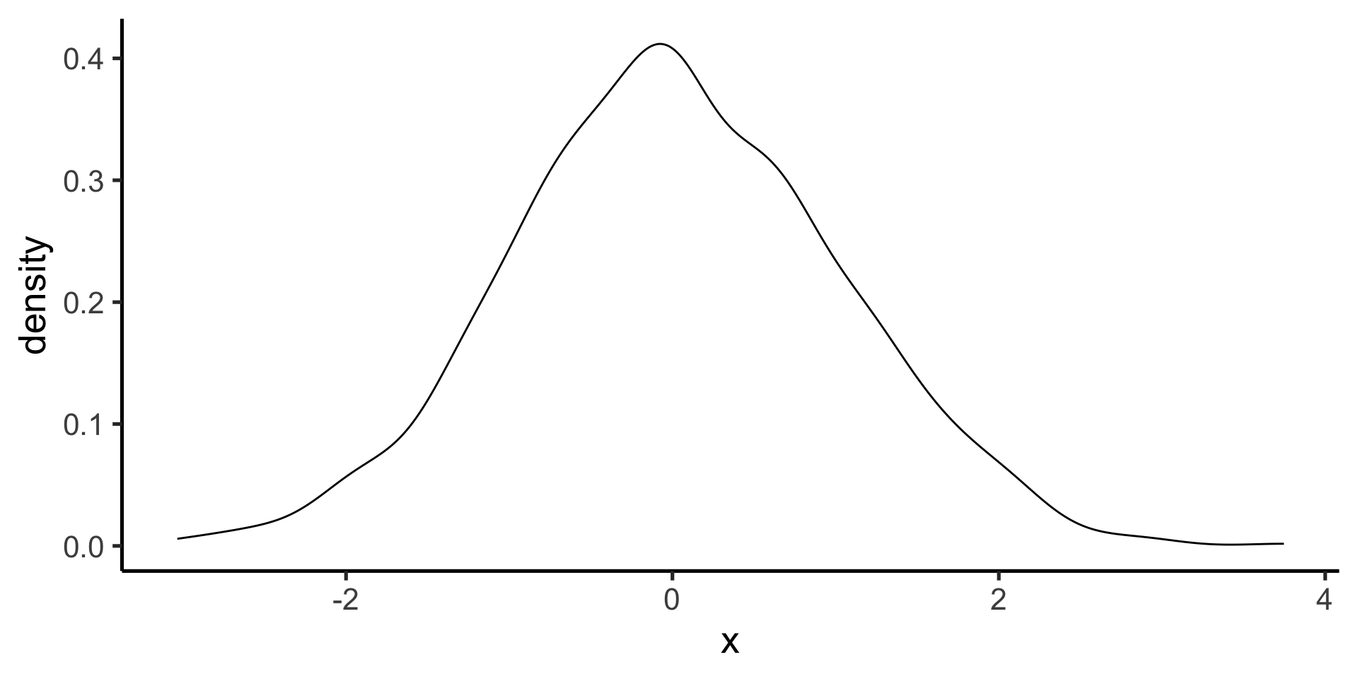
Visualize the distribution

Suppose we have a non-normal distribution

Nonparametric statistics

mean() and sd() are not a good summary of central tendency and variability anymore.

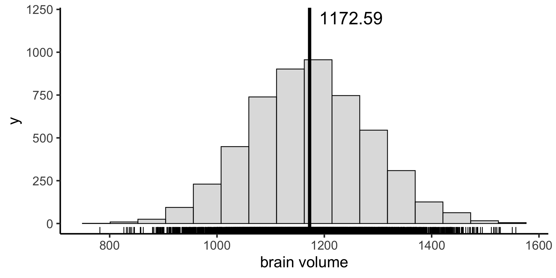
Median

Instead we can use the median as our measure of central tendency: the value below which 50% of the data points fall.

IQR

And the interquartile range (IQR) as a measure of the spread in our data: the difference between the 25th and 75th percentiles (50% of the data fall between these values)

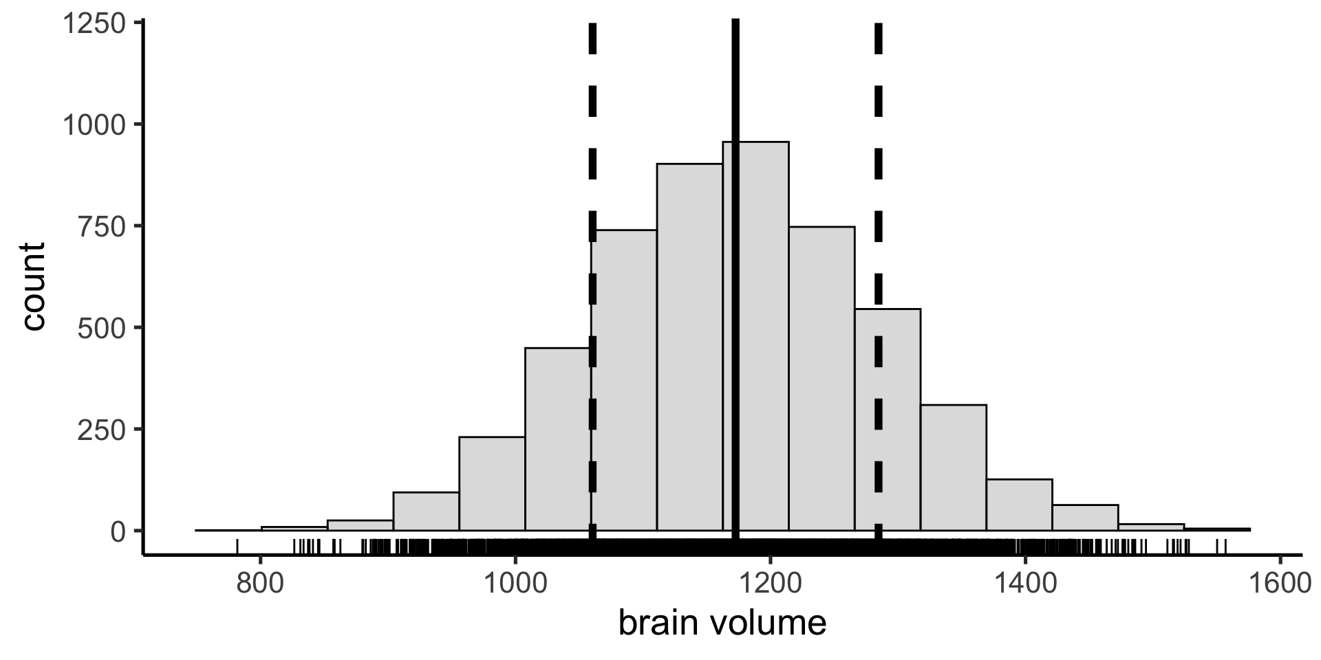
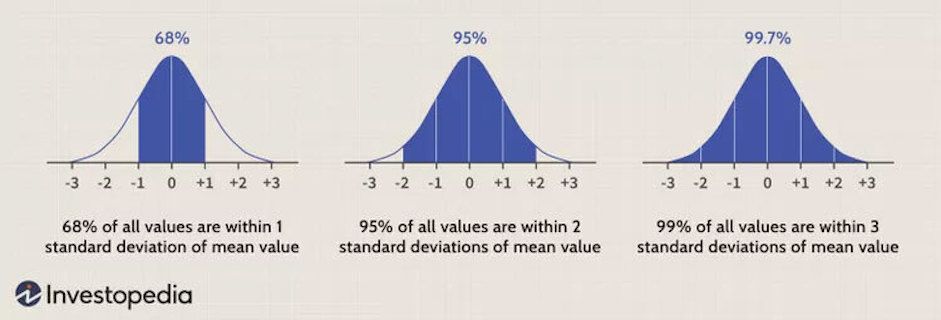
Coverage interval

We can calculate any arbitrary coverage interval. In the sciences we often use the 95% coverage interval — the difference between the 2.5 percentile and the 97.5 percentile — including all but 5% of the data.

Probability distributions

A mathematical function that describes the probability of observing different possible values of a variable (also called probability density function)

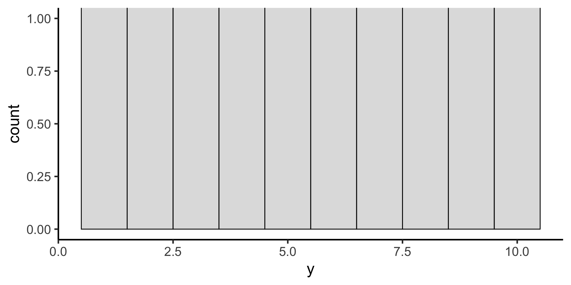
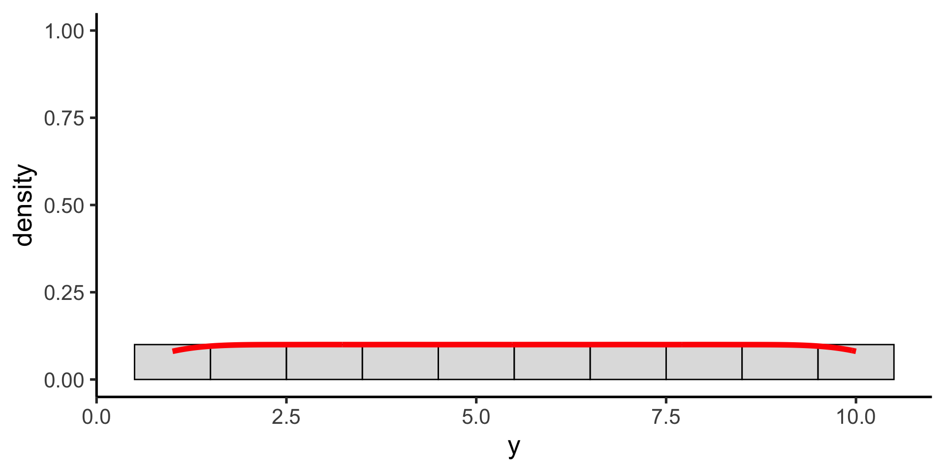
Uniform probability distribution

All possible values are equally likely

\(p(x) = \frac{1}{max-min}\)

The probability density function for the uniform distribution is given by this equation (with two parameters: min and max).

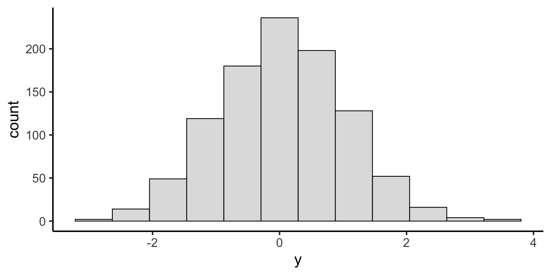
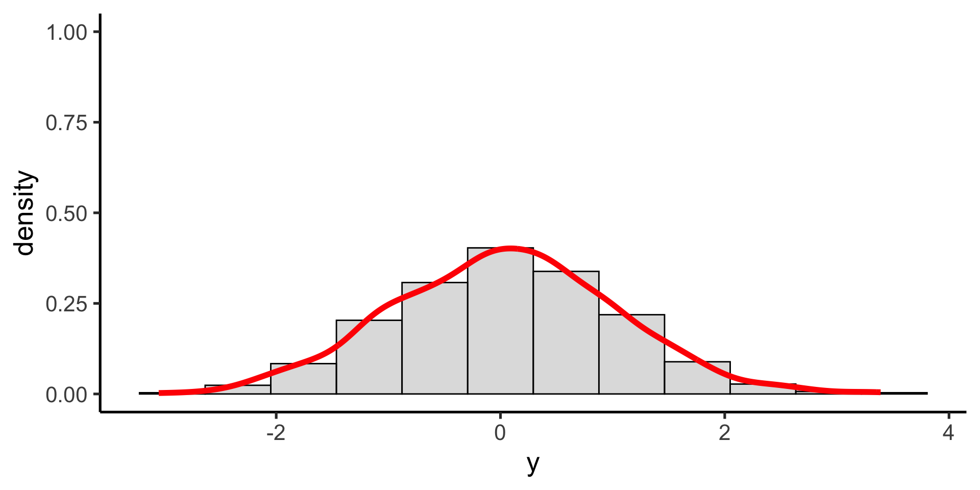
Gaussian (normal) probability distribution

One of the most useful probability distributions for our purposes is the Gaussian (or Normal) distribution

\(p(x) = \frac{1}{\sigma\sqrt{2\pi}}\exp\left(-\frac{1}{2}\left(\frac{x-\mu}{\sigma}\right)^{2}\right)\)

The probability density function for the Gaussian distribution is given by the following equation, with the parameters \(\mu\) (mean) and \(\sigma\) (standard deviation).

Gaussian (normal) probability distribution

• When computing the mean and standard deviation of a set of data, we are implicitly fitting a Gaussian distribution to the data.

Sampling variability

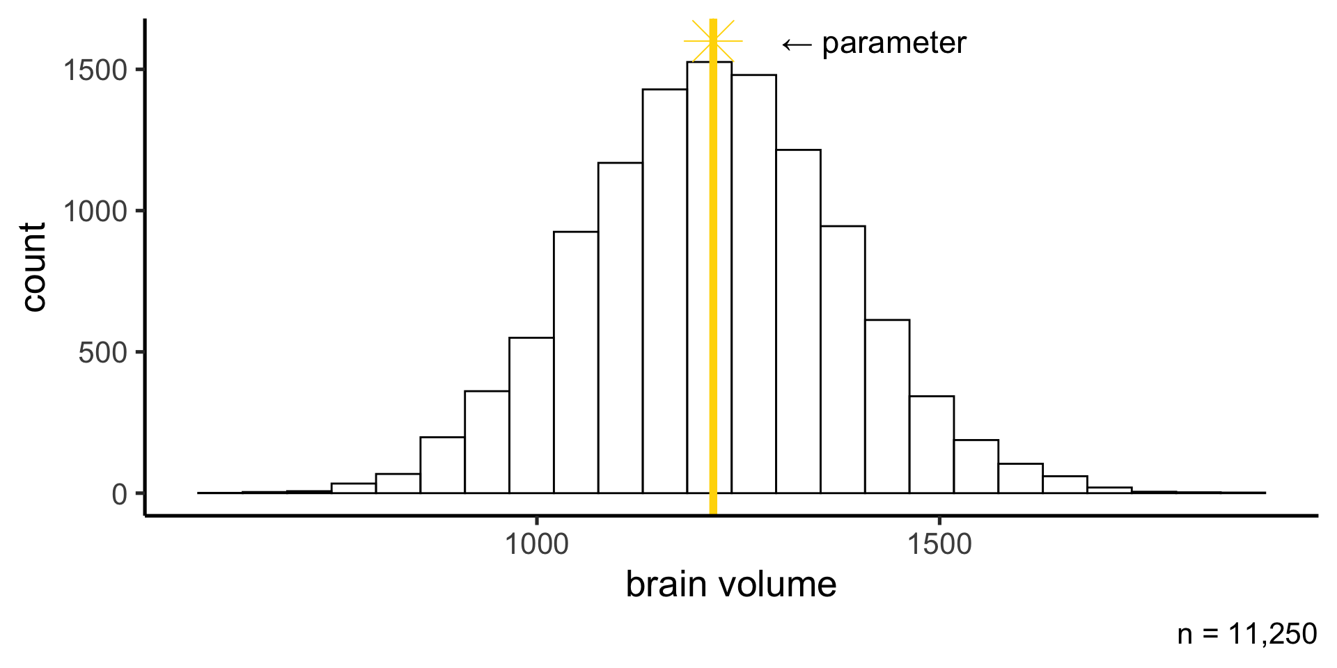
The population

When measuring some quantity, we are usually interested in knowning something about the population: the mean brain volume of Penn undergrads (the parameter)

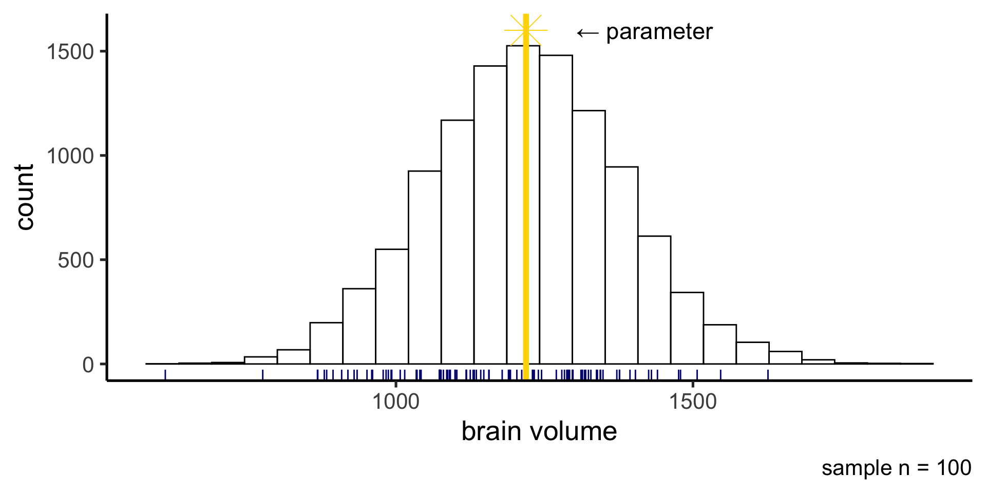
The sample

But we only have a small sample of the population: maybe we can measure the brain volume of 100 students

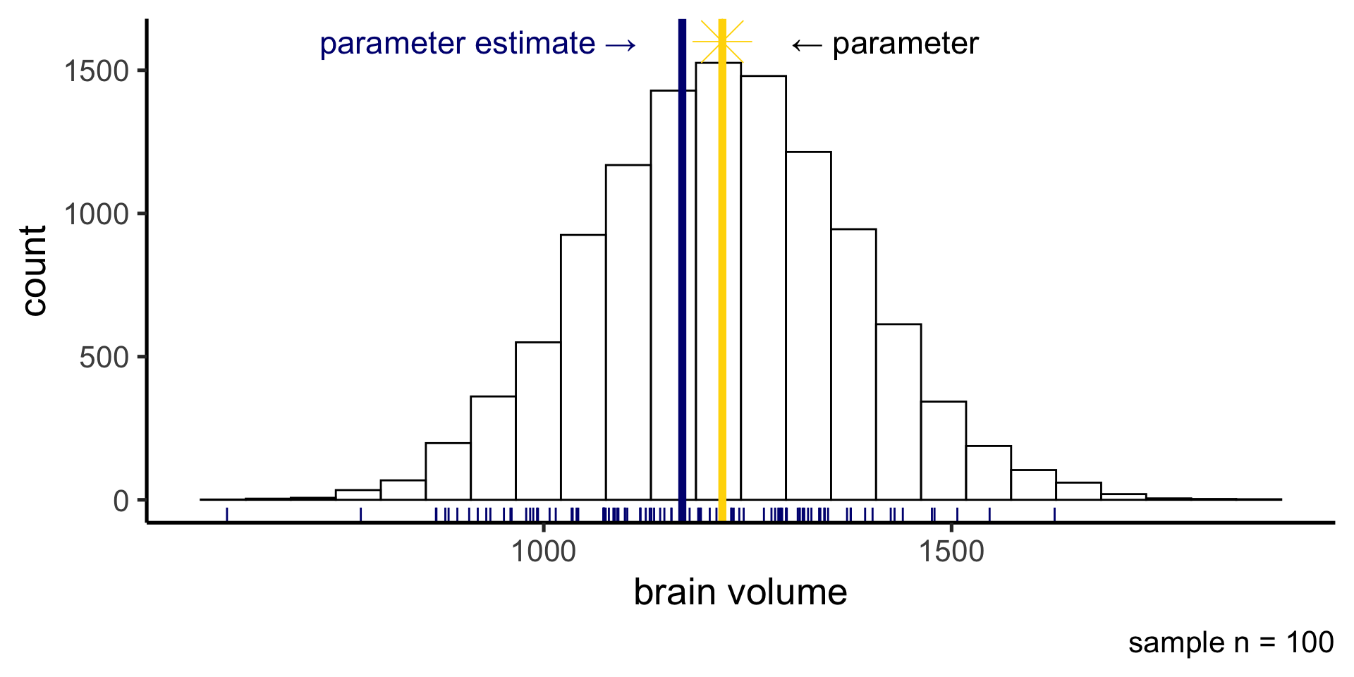
Sampling variability

Any statistic we compute from a random sample we’ve collected (parameter estimate) will be subject to sampling variability and will differ from that statistics computed on the entire population (parameter)

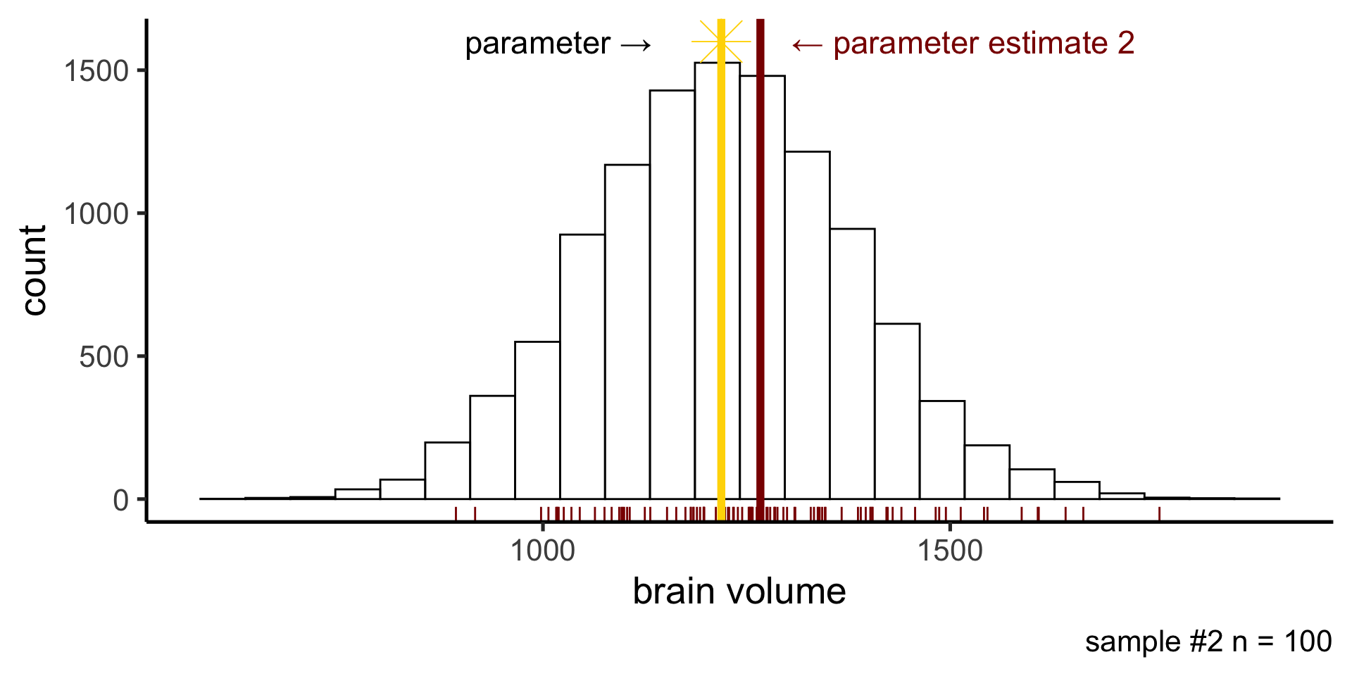
Sampling variability

If we took another sample of 100 students, our parameter estimate would be different.

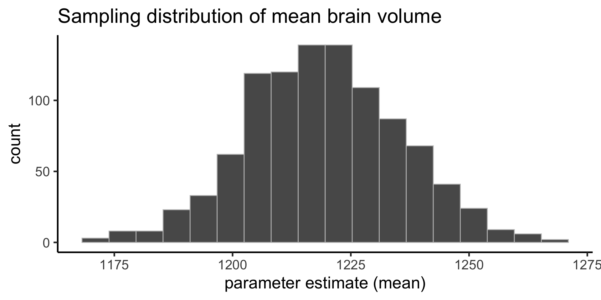
Sampling distribution

The sampling distribution is the probability distribution of values our parameter estimate can take on. Constructed by taking a random sample, computing stat of interest, and repeating many times.

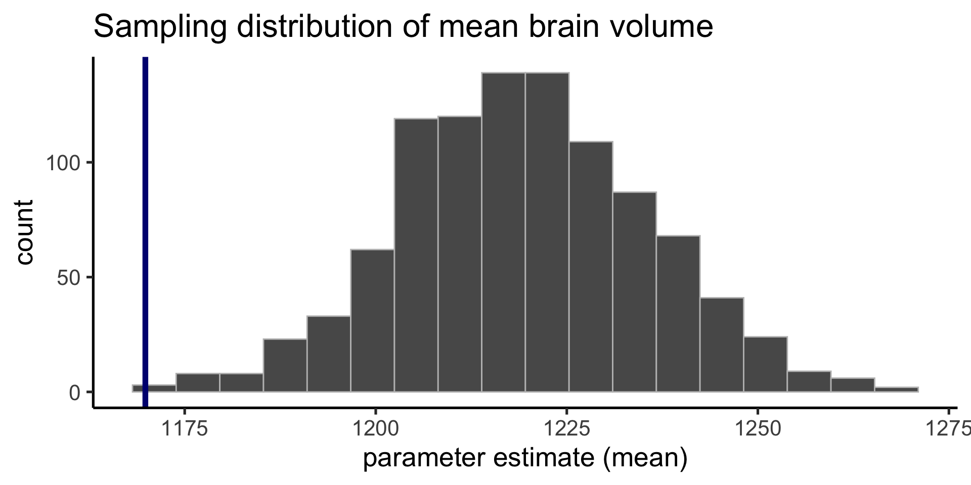
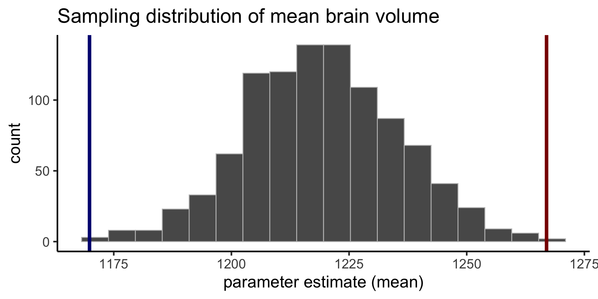
Sampling distribution

Our first sample was on the low end of possible mean brain volume.

Sampling distribution

Our second sample was on the high end of possible mean brain volume.

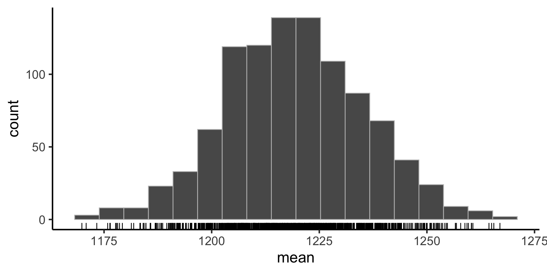
Quantifying sampling variability

The spread of the sampling distribution indicates how the parameter estimate will vary from different random samples.

Quantifying sampling variability

We can quantify the spread (express our uncertainty on our parameter estimate) in two ways.

• Parametrically, by compute the standard error
• Nonparametrically, by constructing a confidence interval

Quantifying sampling variability

One way is to compute the standard deviation of the sampling distribution, which has a special name: the standard error

• The standard error is given by the following equation, where \(\sigma\) is the standard deviation of the population and \(n\) is the sample size.
• \(\frac{\sigma}{n}\)
• In practice, the standard deviation of the population is unknown, so we use the standard deviation of the sample as an estimate.

Standard error is parametric

• Standard error is a parametric statistic because we assume a gaussian probaiblity distribution and compute standard error based on what happens theoretically when we sample from that theoretical distribution.
• \(\frac{\sigma}{n}\)

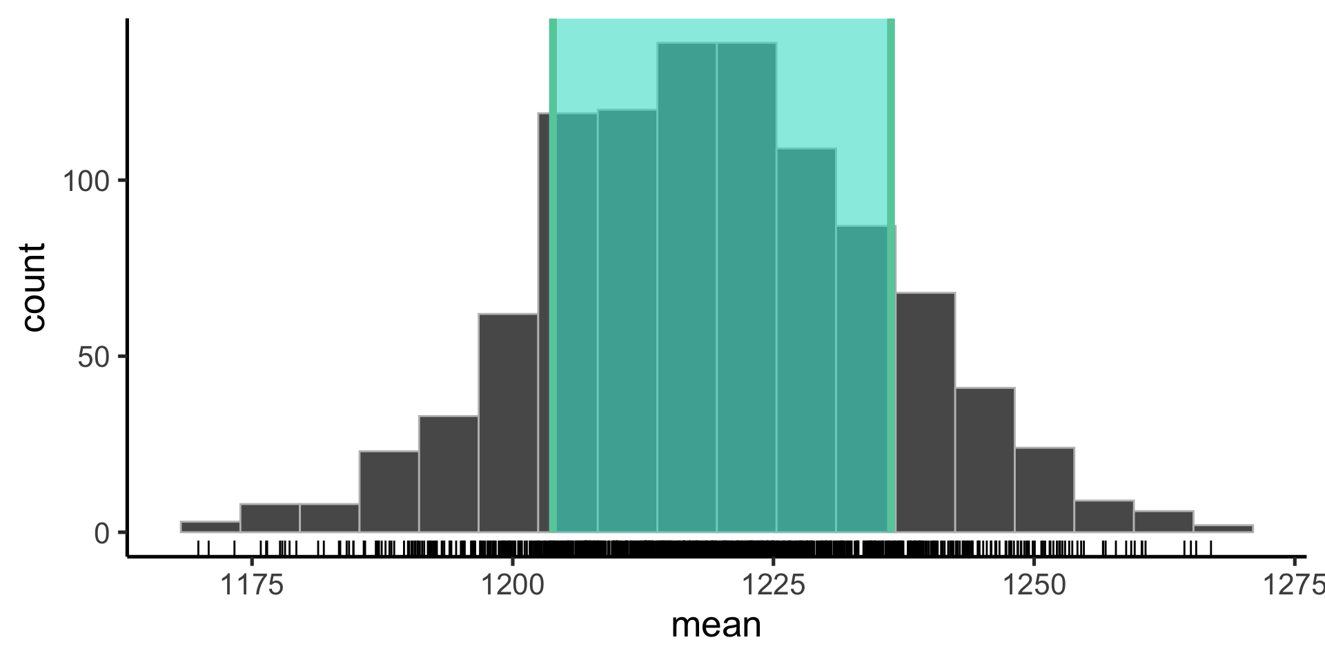
Quantifying sampling variability

Another way is to construct a confidence interval

Practical considerations

• We don’t have access to the entire population
• We can (usually) only do our experiment once
• So, in practice we only have one sample

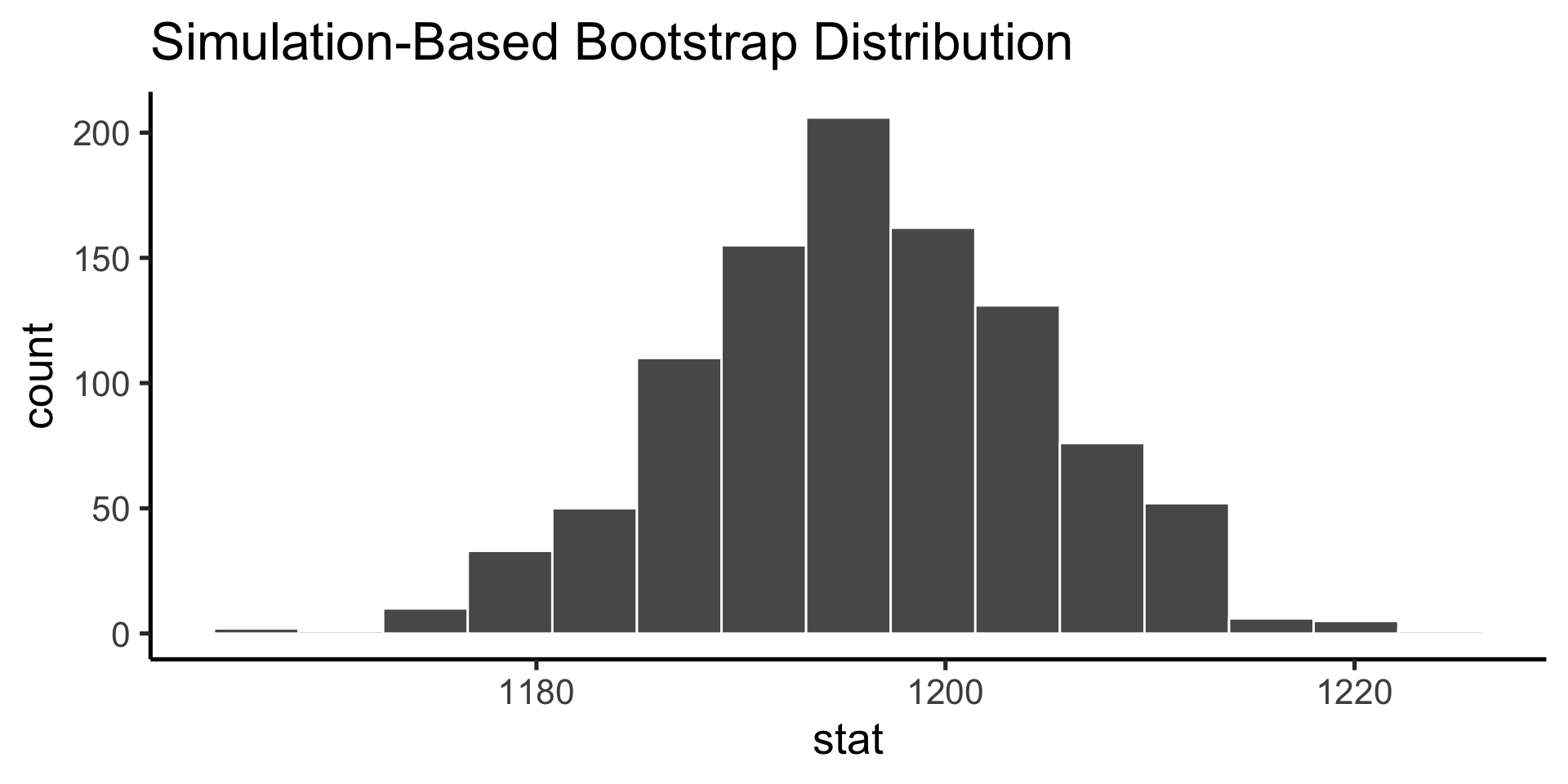
Bootstrapping

To construct the sampling distribution

Bootstrapping

Instead of assuming a parametric probability distributon, we use the data themselves to approximate the underlying distribution: we sample our sample!

Bootsrapping with infer

The objective of this package is to perform statistical inference using an expressive statistical grammar that coheres with the tidyverse design framework

install.packages("infer")`

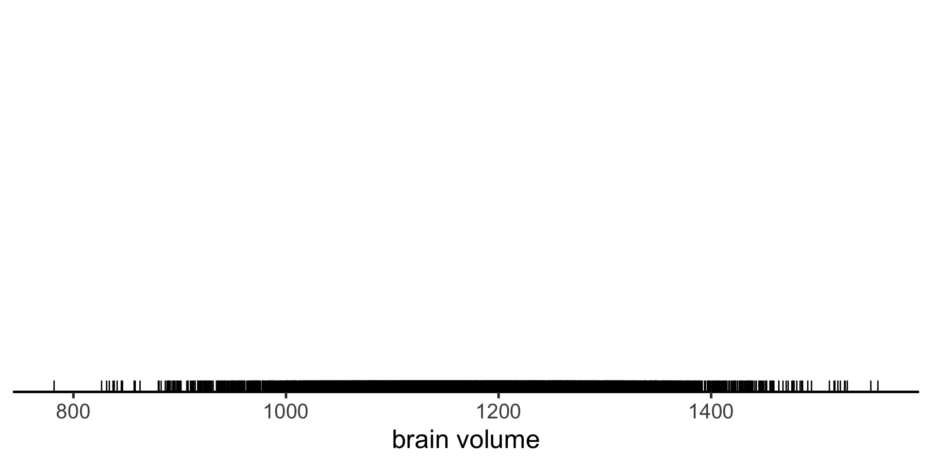
Let’s create some data

Suppose we collect a sample of 100 subjects and find their mean brain volume is 1200 cubic cm and sd is 100:

# get a sample to work with as our "data"
sample1 <- tibble(
  subject_id = 1:100,
  volume = rnorm(100, mean = 1200, sd = 100)
)

sample1 %>% head(10)

# A tibble: 10 × 2
   subject_id volume
        <int>  <dbl>
 1          1  1225.
 2          2  1186.
 3          3  1176.
 4          4  1207.
 5          5  1173.
 6          6  1137.
 7          7  1118.
 8          8  1177.
 9          9  1169.
10         10  1216.

Generate the sampling distribution

Generate the sampling distribution with specify(), generate(), and calculate()

bootstrap_distribution <- sample1  %>% 
  specify(response = volume) %>% 
  generate(reps = 1000, type = "bootstrap") %>% 
  calculate(stat = "mean")

bootstrap_distribution

Response: volume (numeric)
# A tibble: 1,000 × 2
   replicate  stat
       <int> <dbl>
 1         1 1213.
 2         2 1184.
 3         3 1194.
 4         4 1184.
 5         5 1200.
 6         6 1180.
 7         7 1197.
 8         8 1202.
 9         9 1189.
10        10 1193.
# ℹ 990 more rows

Visualize the bootstrap distribution

Visualize the bootstrap distribution you generated with visualize()

bootstrap_distribution %>% 
  visualize()

• Visualize is a shortcut function to ggplot!

Quantify the spread with se

Quantify the spread of the bootstrapped sampling distributon with get_confidence_interval(), and set the type to se for standard error.

se_bootstrap <- bootstrap_distribution %>% 
  get_confidence_interval(
    type = "se",
    point_estimate = mean(sample1$volume)
  )

se_bootstrap

# A tibble: 1 × 2
  lower_ci upper_ci
     <dbl>    <dbl>
1    1179.    1213.

bootstrap_distribution %>% 
  visualize() +
  shade_confidence_interval(
    endpoints = se_bootstrap
  )

Quantify the spread with ci

Quantify the spread of the sampling distributon with get_confidence_interval, and set the type to percentile for confidence interval

ci_bootstrap <- bootstrap_distribution %>% 
  get_confidence_interval(
    type  ="percentile", 
    level = 0.95
  )

ci_bootstrap

# A tibble: 1 × 2
  lower_ci upper_ci
     <dbl>    <dbl>
1    1178.    1212.

bootstrap_distribution %>% 
  visualize() +
  shade_confidence_interval(
    endpoints = ci_bootstrap
  )

Questions?

• Let’s stop there, and work through some more demos in our next lecture!

Thursday

Plan for today

Tuesday’s lecture was conceptual. Today we will demo those concepts to try to understand them better.

Descriptive statistics

Let’s first try to understand descriptive statistics a bit better by using a toy dataset.

Creating a ‘toy’ dataset

Suppose we create a tibble that measures a single quantity: how many minutes your instructor was late to class for 10 days.

(data <- tibble(
  late_minutes = c(1, 2, 2, 3, 4, 2, 5, 3, 3)
))

# A tibble: 9 × 1
  late_minutes
         <dbl>
1            1
2            2
3            2
4            3
5            4
6            2
7            5
8            3
9            3

We can sort the values with arrange to get a quick sense of the data

data %>% 
  arrange(late_minutes) 

# A tibble: 9 × 1
  late_minutes
         <dbl>
1            1
2            2
3            2
4            2
5            3
6            3
7            3
8            4
9            5

Summarize with descriptive statistics

Recall tha twe can summarize (or describe) a set of data with descriptive statistics (aka summary statistics). There are three we typically use:

Measure	Stats	Describes
Central tendency	mean, median, mode	a central or typical value
Variability	variance, standard deviation, range, IQR	dispersion or spread of values
Frequency distribution	count	how frequently different values occur

Frequency distribution

We can create a visual summary of our dataset with a histogram, which plots the frequency distribution of the data.

data %>%
  ggplot(aes(x = late_minutes)) + 
  geom_histogram() 

We can also get a count with group_by() and tally()

data %>% 
  group_by(late_minutes) %>%
  tally() 

# A tibble: 5 × 2
  late_minutes     n
         <dbl> <int>
1            1     1
2            2     3
3            3     3
4            4     1
5            5     1

Central tendency

Measure of central tendency describe where a central or typical value might fall

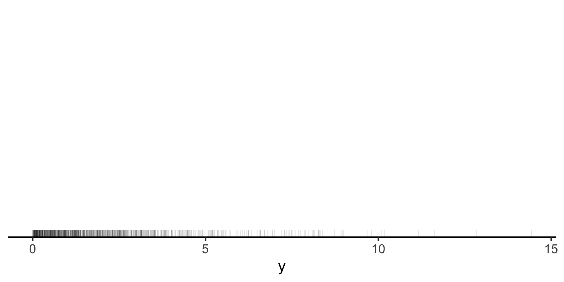
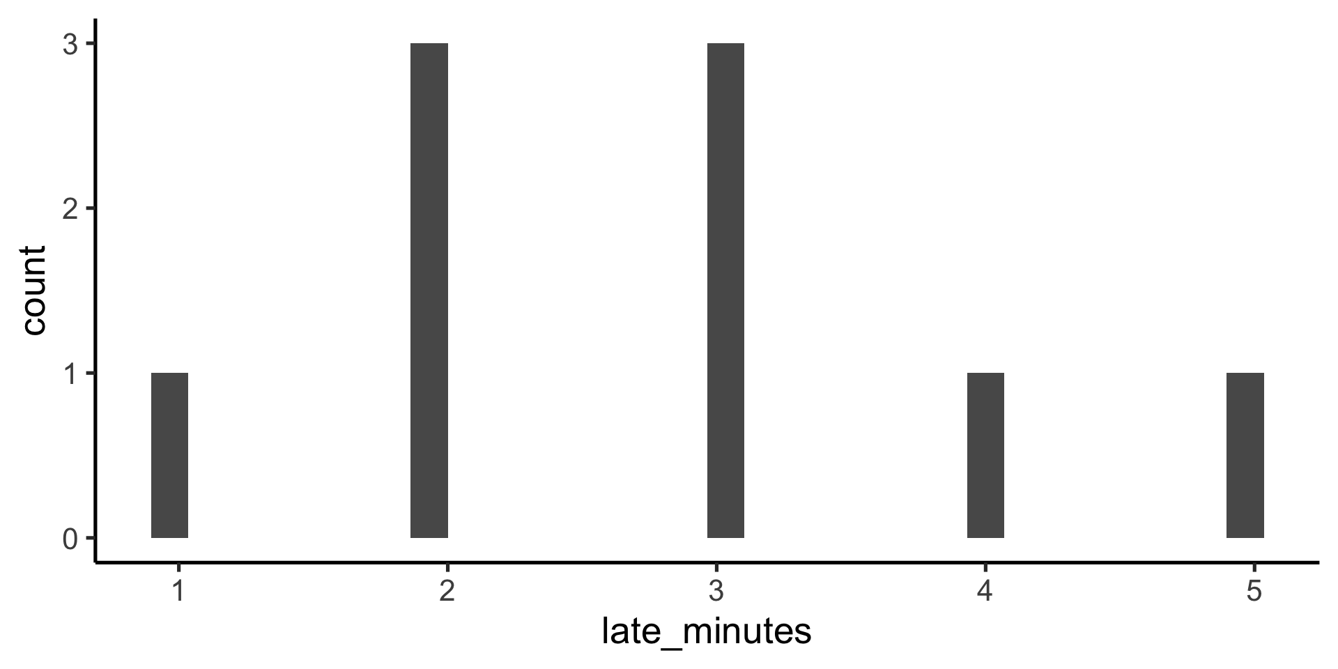
data %>%
  ggplot(aes(x = late_minutes)) + 
  geom_histogram() 

We can get these with group_by() and summarise()

data %>% 
  summarise(
    n = n(), 
    mean = mean(late_minutes), 
    median = median(late_minutes)
    )

# A tibble: 1 × 3
      n  mean median
  <int> <dbl>  <dbl>
1     9  2.78      3

Variability

Measures of variability which describe the dispersion or spread of values

data %>%
  ggplot(aes(x = late_minutes)) + 
  geom_histogram() 

We can also get these with group_by() and summarise()

data %>% 
  summarise(
    n = n(), 
    sd = sd(late_minutes), 
    min = min(late_minutes), 
    max = max(late_minutes), 
    lower = quantile(late_minutes, 0.25),
    upper = quantile(late_minutes, 0.75) 
    )

# A tibble: 1 × 6
      n    sd   min   max lower upper
  <int> <dbl> <dbl> <dbl> <dbl> <dbl>
1     9  1.20     1     5     2     3

Parametric descriptive statistics

Some statistics are considered parametric because they make assumptions about the distribution of the data (we can compute them theoretically from parameters)

Mean

The mean is one example of a parametric descriptive statistic, where \(x_{i}\) is the \(i\)-th data point and \(n\) is the total number of data points

\(mean(x) = \bar{x} = \frac{\sum_{i=i}^{n} x_{i}}{n}\)

mean(data$late_minutes)

[1] 2.777778

We can compute this equation by hand to see that the results are the same.

sum(data$late_minutes)/length(data$late_minutes)

[1] 2.777778

Standard deviation

Standard deviation is another paramteric descriptive statistic where \(x_{i}\) is the \(i\)-th data point, \(n\) is the total number of data points, and \(\bar{x}\) is the mean.

\(sd(x) = \sqrt{\frac{\sum_{i=1}^n (x_i - \bar{x})^2}{n-1}}\)

sd(data$late_minutes)

[1] 1.20185

We can compute this by hand as well, to see how it happens under the hood of sd()

mean_late <- mean(data$late_minutes)
(sd_by_hand <- data %>% 
  mutate(dev = late_minutes - mean_late) %>%
  mutate(sq_dev = dev^2))

# A tibble: 9 × 3
  late_minutes    dev sq_dev
         <dbl>  <dbl>  <dbl>
1            1 -1.78  3.16  
2            2 -0.778 0.605 
3            2 -0.778 0.605 
4            3  0.222 0.0494
5            4  1.22  1.49  
6            2 -0.778 0.605 
7            5  2.22  4.94  
8            3  0.222 0.0494
9            3  0.222 0.0494

sd_by_hand %>% 
  summarise(
    n = n(), 
    n_minus_1 = n-1, 
    sum_sq_dev = sum(sq_dev), 
    by_hand_sd = sqrt(sum_sq_dev/n_minus_1))

# A tibble: 1 × 4
      n n_minus_1 sum_sq_dev by_hand_sd
  <int>     <dbl>      <dbl>      <dbl>
1     9         8       11.6       1.20

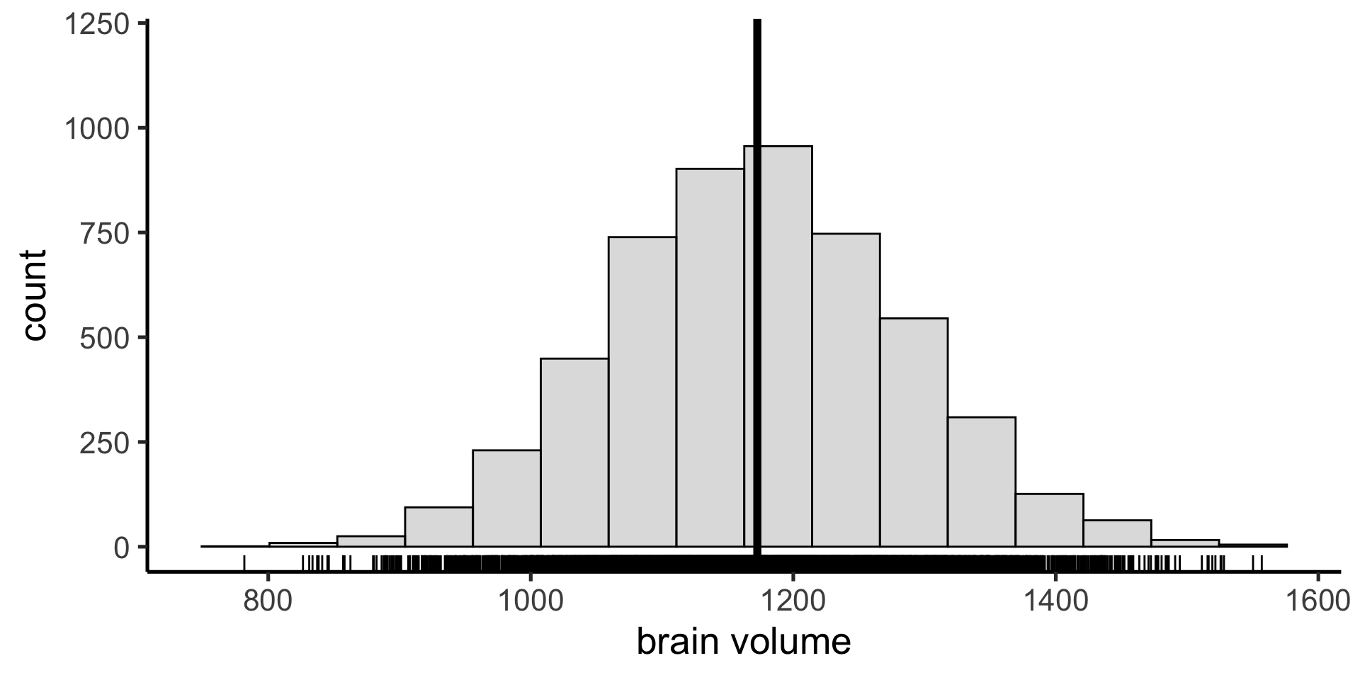
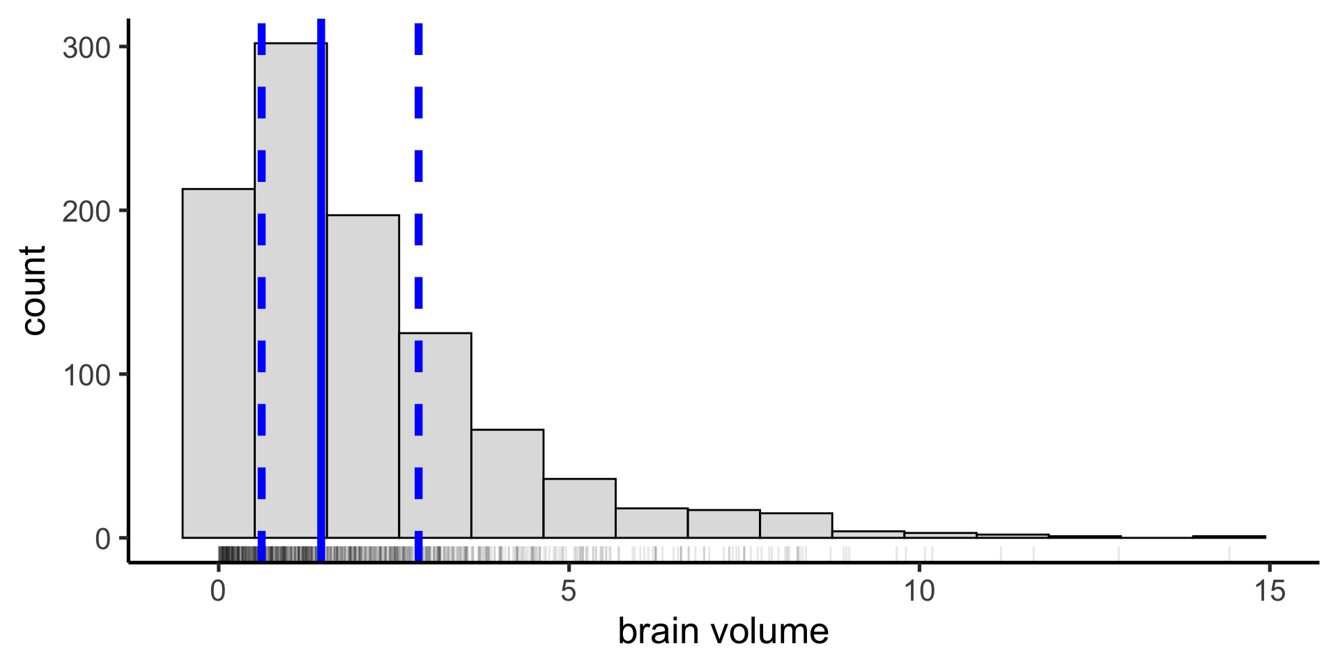
Visualize the mean and sd

How do we visualize the mean and sd on our histogram?

First get the summary statistics with summarise()

(sum_stats <- data %>%
  summarise(
    n = n(), 
    mean = mean(late_minutes), 
    sd = sd(late_minutes), 
    lower_sd = mean - sd, 
    upper_sd = mean + sd
  ))

# A tibble: 1 × 5
      n  mean    sd lower_sd upper_sd
  <int> <dbl> <dbl>    <dbl>    <dbl>
1     9  2.78  1.20     1.58     3.98

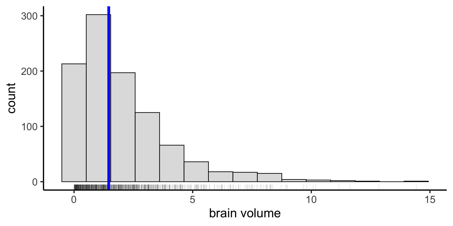
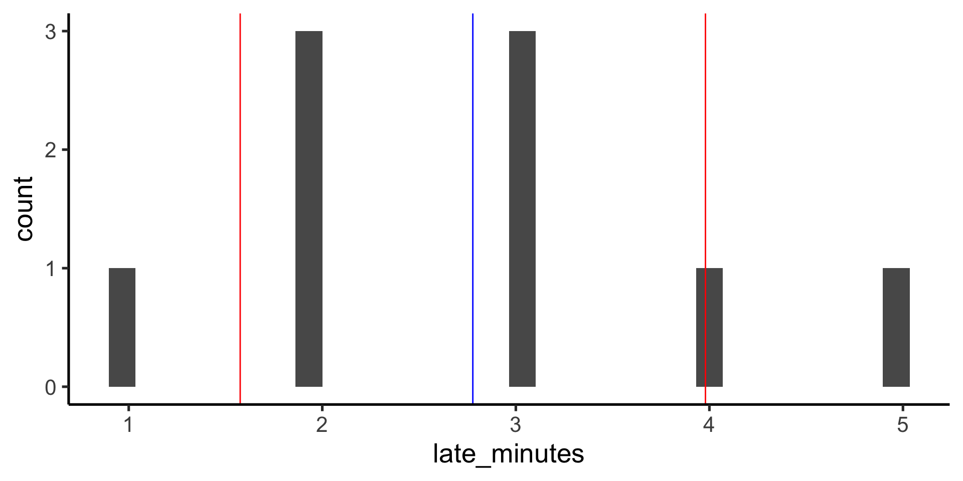
Then use those values to plot with geom_vline().

data %>%
  ggplot(aes(x = late_minutes)) + 
  geom_histogram() +
  geom_vline(
    xintercept = sum_stats$mean, 
    color = "blue"
    ) + 
  geom_vline(
    xintercept = sum_stats$lower_sd,
    color = "red"
    ) +
  geom_vline(
    xintercept = sum_stats$upper_sd, 
    color = "red"
    )

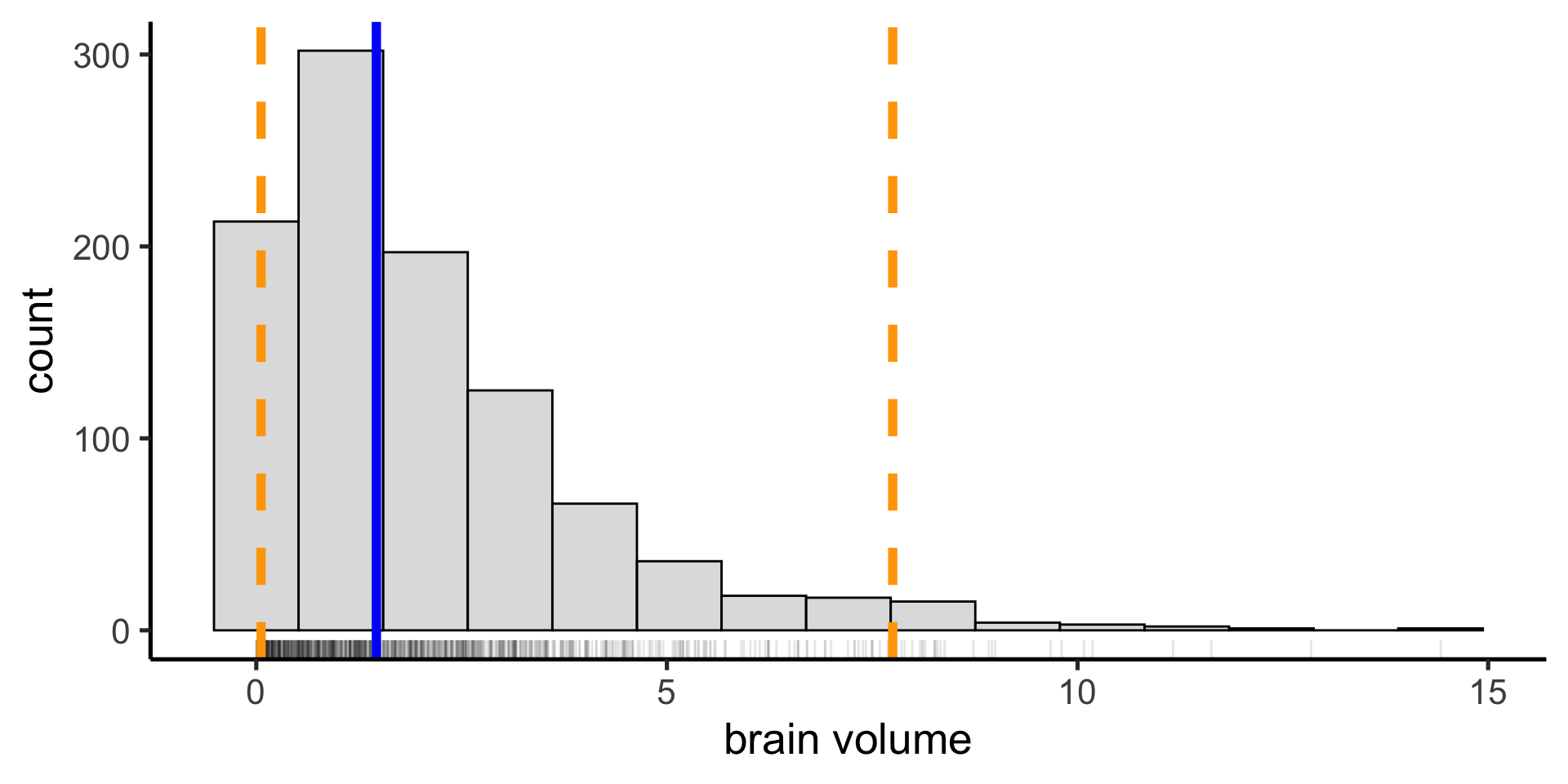
Nonparametric descriptive statistics

Other statistics are considered nonparametric, because thy make minimal assumptions about the distribution of the data (we can compute them theoretically from parameters)

Median

The mean is the value below which 50% of the data fall.

median(data$late_minutes) 

[1] 3

We can check whether this is accurate by sorting our data

data %>% 
  arrange(late_minutes) 

# A tibble: 9 × 1
  late_minutes
         <dbl>
1            1
2            2
3            2
4            2
5            3
6            3
7            3
8            4
9            5

Inter-quartile range (IQR)

The difference between the 25th and 75th percentiles. We can compute these values with the quantile() function.

data %>%
  summarise(
    iqr_lower = quantile(late_minutes, 0.25), 
    iqr_upper = quantile(late_minutes, 0.75)
  )

# A tibble: 1 × 2
  iqr_lower iqr_upper
      <dbl>     <dbl>
1         2         3

Again, we can check whether this is accurate by sorting our data

data %>% 
  arrange(late_minutes) 

# A tibble: 9 × 1
  late_minutes
         <dbl>
1            1
2            2
3            2
4            2
5            3
6            3
7            3
8            4
9            5

Coverage intervals

The IQR is also called the 50% coverage interval (because 50% of the data fall in this range). We can calculate any artibrary coverage interval with quantile()

data %>%
  summarise(
    iqr_lower = quantile(late_minutes, 0.025), 
    iqr_upper = quantile(late_minutes, 0.975)
  )

# A tibble: 1 × 2
  iqr_lower iqr_upper
      <dbl>     <dbl>
1       1.2       4.8

Again, we can check whether this is accurate by sorting our data

data %>% 
  arrange(late_minutes) 

# A tibble: 9 × 1
  late_minutes
         <dbl>
1            1
2            2
3            2
4            2
5            3
6            3
7            3
8            4
9            5

Visualize the median and coverage intervals

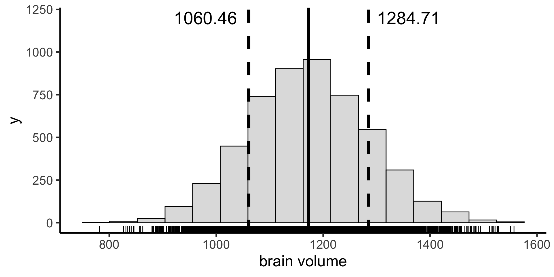
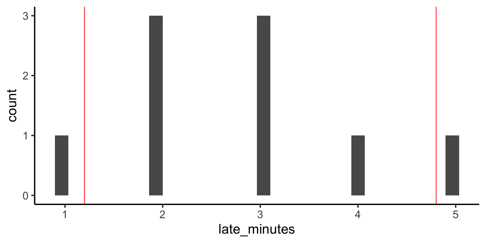
We can visualize these statistics on our histograms in the same way we did mean and sd:

First get the summary statistics with summarise()

(sum_stats <- data %>%
  summarise(
    n = n(), 
    median = median(late_minutes), 
      ci_lower = quantile(late_minutes, 0.025), 
    ci_upper = quantile(late_minutes, 0.975)
  ))

# A tibble: 1 × 4
      n median ci_lower ci_upper
  <int>  <dbl>    <dbl>    <dbl>
1     9      3      1.2      4.8

Then use those values to plot with geom_vline().

data %>%
  ggplot(aes(x = late_minutes)) + 
  geom_histogram() +
  geom_vline(
    xintercept = sum_stats$mean, 
    color = "blue"
    ) + 
  geom_vline(
    xintercept = sum_stats$ci_lower,
    color = "red"
    ) +
  geom_vline(
    xintercept = sum_stats$ci_upper, 
    color = "red"
    )

Probability distributions

A probability distribution is a mathematical function of one (or more) variables that describes the likelihood of observing any specific set of values for the variables.

R’s functions for parametric probability distributions

function	params	returns
d*()	depends on *	height of the probability density function at the given values
p*()	depends on *	cumulative density function (probability that a random number from the distribution will be less than the given values)
q*()	depends on *	value whose cumulative distribution matches the probaiblity (inverse of p)
r*()	depends on *	returns n random numbers generated from the distribution

Uniform distribution

The uniform distribution is the simplest probability distribution, where all values are equally likely. The probability density function for the uniform distribution is given by this equation (with two parameters: min and max).

\(p(x) = \frac{1}{max-min}\)

R’s functions for Gaussian distribution

We just use norm (normal) to stand in for the *

function	params	returns
dnorm()	x, mean, sd	height of the probability density function at the given values
pnorm()	q, mean, sd	cumulative density function (probability that a random number from the distribution will be less than the given values)
qnorm()	p, mean, sd	value whose cumulative distribution matches the probaiblity (inverse of p)
rnorm()	n, mean, sd	returns n random numbers generated from the distribution

rnorm() to sample from the distribution

rnorm(n, mean, sd): returns n random numbers generated from the distribution

(normy <- tibble(
  x = rnorm(1000, mean = 0, sd = 1)
))

# A tibble: 1,000 × 1
         x
     <dbl>
 1  2.16  
 2  0.0405
 3 -1.95  
 4 -1.30  
 5 -0.139 
 6  1.48  
 7  0.346 
 8 -2.22  
 9  0.0657
10  0.367 
# ℹ 990 more rows

dnorm(x, mean, sd)

Returns the height of the probability density function at the given values

ggplot(normy, aes(x = x )) +
  geom_density()

dnorm(2, mean = 0, sd = 1)

[1] 0.05399097

pnorm(q, mean, sd)

Returns the cumulative density function (probability that a random number from the distribution will be less than the given values)

ggplot(normy, aes(x = x )) +
  geom_density()

pnorm(3, mean = 0, sd = 1)

[1] 0.9986501

pnorm(-2, mean = 0, sd = 1)

[1] 0.02275013

qnorm(p, mean, sd)

Returns the value whose cumulative distribution matches the probability

ggplot(normy, aes(x = x )) +
  geom_density()

qnorm(0.99, mean = 0, sd = 1)

[1] 2.326348

qnorm(0.02, mean = 0, sd = 1)

[1] -2.053749

Using other distributions

Change the function’s suffix (the * in r*()) to another distribution and pass the parameters that define that distribution.

runif(n, min, max): returns n random numbers generated from the distribution

(uni<- tibble(
  x = runif(1000, min= 0, max = 1)
))

# A tibble: 1,000 × 1
        x
    <dbl>
 1 1.000 
 2 0.846 
 3 0.0804
 4 0.362 
 5 0.887 
 6 0.0295
 7 0.208 
 8 0.509 
 9 0.299 
10 0.703 
# ℹ 990 more rows

But remember, this only works for paramteric probability distributions (those defined by particular paramters)

Sampling distribution and bootstrapping

Let’s do a walk through from start to finish

The parameter

Generate data for the brain volume of the 28201 grad and undergrad students at UPenn and compute the parameter of interest (mean brain volume)

(population <- tibble(
  subject_id = 1:28201, 
  volume = rnorm(28201, mean = 1200, sd = 100)
))

# A tibble: 28,201 × 2
   subject_id volume
        <int>  <dbl>
 1          1  1166.
 2          2  1262.
 3          3  1312.
 4          4  1038.
 5          5  1084.
 6          6  1355.
 7          7  1275.
 8          8  1036.
 9          9  1238.
10         10  1364.
# ℹ 28,191 more rows

The parameter estimate

Now take a realistic sample of 100 students and compute the paramter estimate (mean brain volume on our sample)

(sample <- population %>%
  sample_n(100))

# A tibble: 100 × 2
   subject_id volume
        <int>  <dbl>
 1      16267  1015.
 2      28046  1363.
 3        952  1318.
 4      22133  1226.
 5       7915  1150.
 6      13497  1045.
 7      11874  1132.
 8      25425  1197.
 9      17087  1170.
10      10368  1235.
# ℹ 90 more rows

But our parameter estimate is noisy

• When measuring a quantity, the measurement will be different each time. We attribute this variability to noise, any factor that contributes variability in measurement.
• Any statistic (e.g. mean) that we compute on a random sample is subject to variability as well; we need to distrust (to some degree) this statistic.
• To indicate our uncertainty on our parameter estimate, we can use
  • standard error (the standard deviation of the sampling distribution; parametric)
  • confidence intervals (the nonparametric approach to quantify spread)

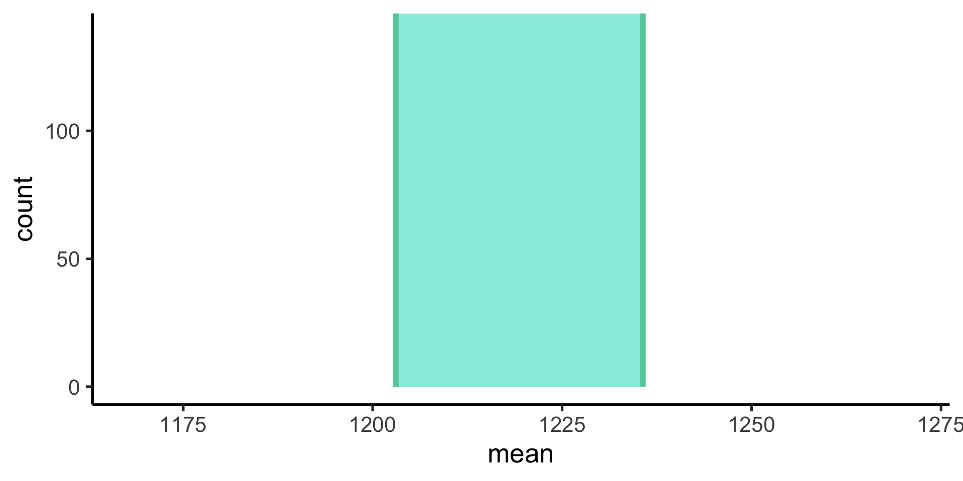
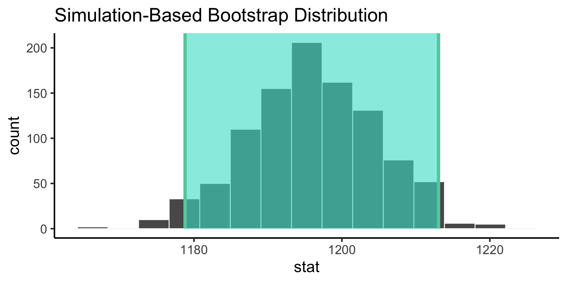
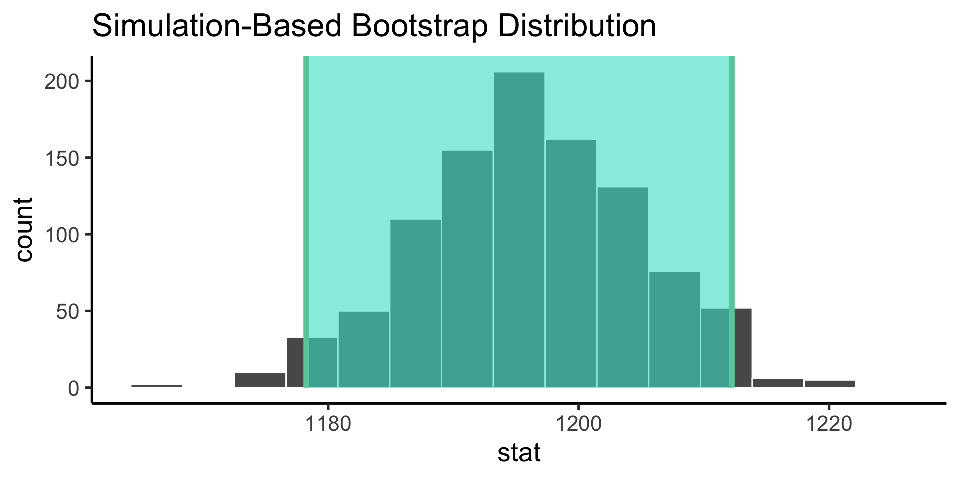
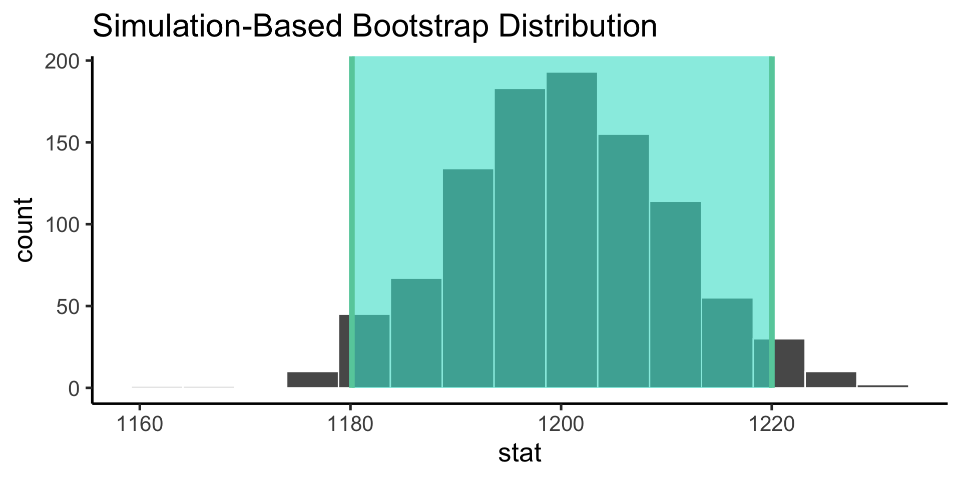
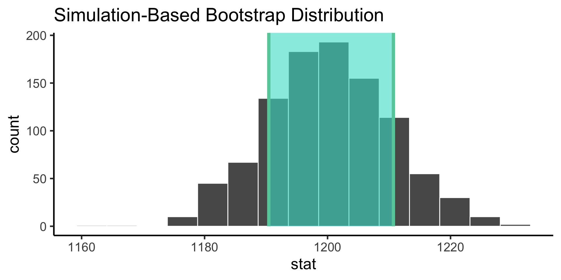
Bootstrap the sampling distribution

Use infer to construct the probability distribution of the values our parameter estimate can take on (the sampling distribution).

(bootstrap_distribution <- sample  %>% 
  specify(response = volume) %>% 
  generate(reps = 1000, type = "bootstrap") %>% 
  calculate(stat = "mean"))

Response: volume (numeric)
# A tibble: 1,000 × 2
   replicate  stat
       <int> <dbl>
 1         1 1203.
 2         2 1199.
 3         3 1209.
 4         4 1200.
 5         5 1195.
 6         6 1197.
 7         7 1200.
 8         8 1218.
 9         9 1195.
10        10 1196.
# ℹ 990 more rows

Standard error

Recall that standard error is the standard deviation of the sampling distribution. It indicaes about how far away the true population might be.

(se_bootstrap <- bootstrap_distribution %>% 
  get_confidence_interval(
    type = "se",
    point_estimate = mean(sample$volume)
  ))

# A tibble: 1 × 2
  lower_ci upper_ci
     <dbl>    <dbl>
1    1180.    1220.

bootstrap_distribution %>% 
  visualize() +
  shade_confidence_interval(
    endpoints = se_bootstrap
  )

Confidence interval

Confidence intervals are the nonparameteric approach to the standard error: if the distribution is Gaussian, +/- 1 standard error gives the 68% confidence internval and +/- 2 gives the 95% confidence interval.

(ci_bootstrap <- bootstrap_distribution %>% 
  get_confidence_interval(
    type = "percentile",
   level = 0.68
  ))

# A tibble: 1 × 2
  lower_ci upper_ci
     <dbl>    <dbl>
1    1190.    1211.

bootstrap_distribution %>% 
  visualize() +
  shade_confidence_interval(
    endpoints = ci_bootstrap
  )

Interpreting confidence intervals

bootstrap_distribution %>% 
  visualize() +
  shade_confidence_interval(
    endpoints = ci_bootstrap
  )

• technical interpretation: if we repeated our experiment, we can expect the X% of the time, the true population parameter will be contained within the X% confidence interval.
• looser interpretation: we can use the confidence interval as an indicator of our uncertainty in our parameter estimate.

Questions?